Evaluation Metrics for Machine Learning Models with Codes in Python

For assessing a machine learning model's effectiveness, evaluation is essential. A model developed from machine learning is evaluated using a variety of measures. To optimize a model on the basis of performance, choosing the best metrics is crucial. We go through the mathematical foundation and use of evaluation metrics in the classification models in this tutorial.

By creating an ML classification model, we can begin talking about assessment criteria. Here, we have used a random forest classification model on the breast cancer data from the built-in datasets of the Sklearn library.

To set up the appropriate environment, first, we need to import the essential libraries and modules. Then we will load the data and split it into the training and testing data. We will build the model and calculate various accuracy metrics.

Classification Metrics

We will see the metrics we can use to evaluate the classification machine learning models.

Classification Accuracy

The percentage of correctly predicted events to all predicted events is known as classification accuracy.

This assessment metric is often misused when used for categorization problems. It is actually only appropriate if there the observations of each class are equal in number (which seldom occurs) and if all forecasts and prediction errors have an equal weight, which frequently isn't the case.

Here is an illustration of how classification accuracy is determined.

Code

# Python program to see how to calculate classification accuracy evaluation metrics

# We will import the required packages and classes
from sklearn.datasets import load_breast_cancer
from sklearn import metrics
from sklearn.model_selection import train_test_split, KFold, cross_val_score
from sklearn.ensemble import RandomForestClassifier
import pandas as pd

# Importing the Breast Cancer dataset
df = load_breast_cancer()

# Seperating the dependent and independent variables
X = pd.DataFrame(df['data'], columns = df['feature_names'])
y = abs(pd.Series(df['target']) - 1)

# Separating the dataset into the training and the testing dataset in the 80:20 ratio
X_train, X_test, y_train, y_test = train_test_split(X, y, test_size = 0.2, random_state = 1)

# Dividing the training data into ten datasets to perform cross-validation
kfold = KFold(n_splits = 10, random_state = 7, shuffle = True)

# Creating an instance of the model
rfc = RandomForestClassifier(random_state=1)
scoring = 'accuracy'

# Performing cross-validation on the training dataset
results = cross_val_score(rfc, X, y, cv = kfold, scoring = scoring)
print(f"The accuracy matrix is: {results}")
print(f"The mean accuracy is: {results.mean()}, and the standard deviation is: {results.std()}")

Output

The accuracy matrix is: [0.98245614 0.98245614 0.94736842 0.96491228 0.94736842 0.94736842
 0.94736842 0.96491228 0.98245614 0.96428571]
The mean accuracy is: 0.963095238095238, and the standard deviation is: 0.014566692235547473

As we can see, using the cross_val_score function, we can get the mean accuracy score and standard deviation of the accuracy score.

Log Loss

Another evaluation metric is Logistic Loss, also called Log Loss (short form). This metric evaluates the predictions of the probabilities of the target classes belonging to a certain class.

The probability range is [0, 1]. However, Log Loss is the negative average of this probability value. Therefore, a smaller value of log loss is better than the higher value of the log loss. It measures the confidence of the algorithm in predicting or classifying the attributes in different classes. Correct predictions are awarded, and the incorrect predictions are degraded to measure this confidence value.

Below is the code to find the log loss value of a classifier in Python language. We will use the diabetes dataset and Support Vector Classifier to classify the data.

Code

# Python program to show how to calculate the Log Loss value of a model
	
# We will import the required packages and classes
from sklearn.datasets import load_iris
from sklearn.model_selection import train_test_split, KFold, cross_val_score
from sklearn.svm import SVC
import pandas as pd
from sklearn import metrics

# Importing the Iris dataset
df = load_iris()

# Seperating the dependent and independent variables
X = pd.DataFrame(df['data'], columns = df['feature_names'])
y = abs(df['target'] - 1)

# Separating the dataset into the training and the testing dataset in the 70:30 ratio
X_train, X_test, y_train, y_test = train_test_split(X, y, test_size = 0.3, random_state = 1)

# # Dividing the training data into ten datasets to perform cross-validation
# kfold = KFold(n_splits = 10, random_state = 7, shuffle = True)

# Creating an instance of the model
svc = SVC(random_state=1, probability=True)
svc.fit(X_train, y_train)
Y_pred = svc.predict_proba(X_test)
ll = metrics.log_loss(y_test, Y_pred)
print(ll)

Output

0.10352623753628318

The closer the log loss value is to 0, the better the model. 0 is the perfect log loss score.

The random nature of the model or assessment process, as well as variations in numerical precision, may cause your findings to differ. Think about executing this scenario a couple of times and contrasting the typical result.

Area Under ROC Curve

Area Under ROC Curve, or the abbreviated form AUC-ROC, is a performance metric used to evaluate binary classification problems.

The AUC value represents the ability of a classification model to classify the positive and negative classes. The area equal to 1 means the model correctly classified all the attributes. And an area equal to 0.5 means the model randomly classifies the model. A value less than that means that the model is biased for a certain class.

The plot of the true positive value and the false positive values for the given set of probability predictions used to map the probabilities of belonging to a certain class is called a ROC curve. The area under the boundaries of the ROC curve is an approximate definite integral of the function of the curve.

Below is the code to show how to calculate AUC-ROC using Python.

Code

# Python program to see how to calculate AUC-ROC for a trained model

# We will import the required packages and classes
from sklearn.datasets import load_iris
from sklearn.svm import SVC
from sklearn.model_selection import train_test_split
import pandas as pd
from sklearn import metrics

# Importing the Iris dataset
df = load_iris()

# Seperating the dependent and independent variables
X = pd.DataFrame(df['data'], columns = df['feature_names'])
y = abs(df['target'] - 1)

# Separating the dataset into the training and the testing dataset in the 70:30 ratio
X_train, X_test, y_train, y_test = train_test_split(X, y, test_size = 0.3, random_state = 1)

# Creating an instance of the model
svc = SVC(random_state=1, probability=True)
svc.fit(X_train, y_train)
Y_pred = svc.predict_proba(X_test)
auc = metrics.roc_auc_score(y_test, Y_pred[:, 1])
print(auc)

Output

0.9979423868312757

Since the auc_roc_score value is very close to 1, that means the model has almost perfectly classified the classes of the dataset.

Confusion Matrix

The confusion matrix is a representation of the accuracy of the classification model. The model can classify more than two classes. The table has the predictions made by the model on the x-axis and the actual value of the prediction on the y-axis. The cells of the confusion matrix give the count of the predictions made by the classification model.

For instance, the classification model can predict positive and negative, and each prediction can have the values positive and negative. The number of times the model predicted an attribute as negative when it was actually negative comes in the cell prediction = negative and actual = negative. However, the number of times the model predicted and attributed to be positive when it was actually positive comes in the cell prediction = positive and actual = positive.

Here is a representation of the confusion matrix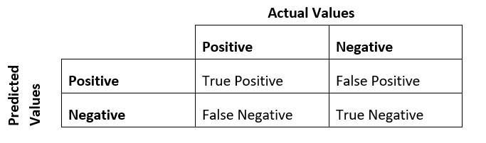

Evaluation Metrics for Machine Learning Models with Codes in Python

True Positive: - This is the number of times the model predicted an independent variable as positive when the actual value was positive.

False Positive: - This is the number of times the model predicted an independent variable as positive when the actual value was negative.

True Negative: - This is the number of times the model predicted an independent variable as negative when the actual value was negative.

False Negative: - This is the number of times the model predicted an independent variable as negative when the actual value was positive.

Here is the code showing how to calculate the confusion matrix in Python for a classification model.

Code

# Python program to see how to calculate the confusion matrix

# We will import the required packages and classes
from sklearn.datasets import load_iris
from sklearn.svm import SVC
from sklearn.model_selection import train_test_split, cross_val_score
import pandas as pd
from sklearn import metrics

# Importing the Iris dataset
df = load_iris()

# Seperating the dependent and independent variables
X = pd.DataFrame(df['data'], columns = df['feature_names'])
y = abs(df['target'] - 1)

# Separating the dataset into the training and the testing dataset in the 70:30 ratio
X_train, X_test, y_train, y_test = train_test_split(X, y, test_size = 0.3, random_state = 1)

# Creating an instance of the model
svc = SVC()
svc.fit(X_train, y_train)
Y_pred = svc.predict(X_test)
matrix = metrics.confusion_matrix(y_test, Y_pred)
print("The confusion matrix is: \n", matrix)

Output

The confusion matrix is:
 [[17 1]
 [ 1 26]]

There is a large number of True Positive and True Negative predictions. Only two predictions are False Negative and False Positive. This means the model is very efficient in correctly classifying the target classes.

Classification Report

Sklearn has a feature of a classification report when we are working with classification models. The report gives a summary of the accuracy of the classification model that we have used to classify the dataset.

The function classification_report() gives the precision value, recall, F1 score, and support values of each class.

Below is the Python code snippet to show how to print this classification report.

Code

# Python program to see how to print the classification report

# We will import the required packages and classes
from sklearn.datasets import load_iris
from sklearn.svm import SVC
from sklearn.model_selection import train_test_split, cross_val_score
import pandas as pd
from sklearn import metrics

# Importing the Iris dataset
df = load_iris()

# Seperating the dependent and independent variables
X = pd.DataFrame(df['data'], columns = df['feature_names'])
y = abs(df['target'] - 1)

# Separating the dataset into the training and the testing dataset in the 70:30 ratio
X_train, X_test, y_train, y_test = train_test_split(X, y, test_size = 0.3, random_state = 1)

# Creating an instance of the model
svc = SVC()
svc.fit(X_train, y_train)
Y_pred = svc.predict(X_test)
report = metrics.classification_report(y_test, Y_pred)
print(report)

Output

              precision    recall  f1-score   support

           0       0.94      0.94      0.94        18
           1       0.96      0.96      0.96        27

    accuracy                           0.96        45
   macro avg       0.95      0.95      0.95        45
weighted avg       0.96      0.96      0.96        45

Precision and Recall

Precision and Recall are two metrics that are like two sides of the same coin. Precision is calculated by dividing the total number of true positive predictions by the total number of positive predictions, i.e., the sum of true positives and false positives. False positives are the incorrect predictions that the model made by predicting the attributes as positives when they actually are negatives.

Recall is another metric that has the power to determine all the relevant instances of a class, that is, all the relevant positive classes and all the relevant negative classes. While precision represents the proportion of the instances of a class according to the model, the recall tells the true proportion of these instances.

As we have said, precision and recall are the two sides of the same coin, and this is because if we make all false positives as true positives, the precision will be one, but the recall will be very low because there will be false negatives also. However, it will go the other way and make all false negatives the positives, the recall will be one, but the precision will be very low. Hence, in simple terms, if we increase precision, the recall will decrease, and if the recall will increase, the precision will decrease.

Code

# Python program to see how to calculate the R-squared error

# We will import the required packages and classes
import numpy as np
from sklearn.datasets import load_breast_cancer
from sklearn.model_selection import train_test_split
from sklearn.svm import SVC
import pandas as pd
from sklearn import metrics

# Importing the Breast Cancer dataset
df = load_breast_cancer()

# Seperating the dependent and independent variables
X = pd.DataFrame(df['data'], columns = df['feature_names'])
y = df['target']

# Separating the dataset into the training and the testing dataset in the 70:30 ratio
X_train, X_test, y_train, y_test = train_test_split(X, y, test_size = 0.3, random_state = 1)

# Creating an instance of the model
svc = SVC()
svc.fit(X_train, y_train)
Y_pred = svc.predict(X_test)
precision = metrics.precision_score(y_test, Y_pred)
print("The precision score is: ", precision)
recall = metrics.recall_score(y_test, Y_pred)
print("The recall score is: ", recall)

Output

The precision score is: 0.8983050847457628
The recall score is: 0.9814814814814815

F1-Score

In some cases, we may need to maximize either the recall score or the precision score at the cost of the remaining one. For instance, in the screening of disease in the patients for further examinations, we will probably want the recall score to be near 1. That is, we will wish to classify all the patients that actually have the disease and have to accept a very low value of precision, which means that we will misclassify some patients as diseased when they will actually not have the disease. However, in this case, there should be an optimum blend of the precision and recall scores. For such scenarios, we can combine the two metrics into one called the F1 score.

The F1 score is calculated by calculating the harmonic mean of the two score values.

We use the harmonic mean against the simple average for a reason. Harmonic means have the power to punish the extremities of the variables. A classification model having a precision score of 1 and the recall score of 0 will have a simple average of 0.5. However, the F1 score, in this case, will be 0. For the F1 score, both the measures carry equal weight, and it is a particular instance of the more general F-beta metric where we can adjust beta to give a desired weight value to either of the measures. We have to maximize the F1 score if we wish to build a classifier with the optimum balance of precision and recall.

Code

# Python program to see how to calculate the F1 score

# We will import the required packages and classes
import numpy as np
from sklearn.datasets import load_breast_cancer
from sklearn.model_selection import train_test_split
from sklearn.svm import SVC
import pandas as pd
from sklearn import metrics

# Importing the Breast Cancer dataset
df = load_breast_cancer()

# Seperating the dependent and independent variables
X = pd.DataFrame(df['data'], columns = df['feature_names'])
y = df['target']

# Separating the dataset into the training and the testing dataset in the 70:30 ratio
X_train, X_test, y_train, y_test = train_test_split(X, y, test_size = 0.3, random_state = 1)

# Creating an instance of the model
svc = SVC()
svc.fit(X_train, y_train)
Y_pred = svc.predict(X_test)
f1 = metrics.f1_score(y_test, Y_pred)
print("The F1 score is: ", f1)

Output

The F1 score is: 
0.9380530973451328

Regression Metrics

In this section, we will review the metrics that we can use to evaluate the regression models.

Mean Absolute Error

The MAE is the mean of the absolute value of the predicted minus the actual values. The error term gives an idea of how wrong predictions are made by the model.

The measure is the magnitude of the error in the predicted values. But the value does not tell the direction of this error. That means it does not tell if the values are over-predicted or are they under-predicted.

Below is the code showing how to determine the value of the mean absolute error in Python. We will use the dataset to fit the linear regression model.

Code

# Python program to see how to calculate the mean absolute error

# We will import the required packages and classes
from sklearn.linear_model import LinearRegression
from sklearn.datasets import load_diabetes
from sklearn.model_selection import train_test_split
import pandas as pd
from sklearn import metrics

# Importing the Diabetes dataset
df = load_diabetes()

# Seperating the dependent and independent variables
X = pd.DataFrame(df['data'], columns = df['feature_names'])
y = abs(df['target'] - 1)

# Separating the dataset into the training and the testing dataset in the 70:30 ratio
X_train, X_test, y_train, y_test = train_test_split(X, y, test_size = 0.3, random_state = 1)

# Creating an instance of the model
lr = LinearRegression()
lr.fit(X_train, y_train)
Y_pred = lr.predict(X_test)
mae = metrics.mean_absolute_error(y_test, Y_pred)
print(mae)

Output

41.64919844144016

The 0 value of MAE suggests that the model had no error in predictions or that it perfectly predicted the values.

We calculate MAE using the mean_absolute _error function of the metrics package.

Mean Squared Error

The Mean Squared Error is similar to the mean absolute error that we calculated above. This metric also provides a net idea of the measurement of error in the predicted values.

We calculate MSE by taking the square root of the mean of the squared of the error terms. This converts the unit of the error back to the unit of the output value and can provide a meaningful description of the predicted values. This error is called the Root Mean Squared Error(RMSE).

Below is the Python code which shows how to determine the value of the mean squared error.

Code

# Python program to see how to calculate the mean squared error

# We will import the required packages and classes
import numpy as np
from sklearn.linear_model import LinearRegression
from sklearn.datasets import load_diabetes
from sklearn.model_selection import train_test_split
import pandas as pd
from sklearn import metrics

# Importing the Diabetes dataset
df = load_diabetes()

# Seperating the dependent and independent variables
X = pd.DataFrame(df['data'], columns = df['feature_names'])
y = df['target']

# Separating the dataset into the training and the testing dataset in the 70:30 ratio
X_train, X_test, y_train, y_test = train_test_split(X, y, test_size = 0.3, random_state = 1)

# Creating an instance of the model
lr = LinearRegression()
lr.fit(X_train, y_train)
Y_pred = lr.predict(X_test)
mse = metrics.mean_squared_error(y_test, Y_pred)
print("Mean Squared Error: ", mse)
print("Root Mean Squared Error: ", np.sqrt(mse))

Output

Mean Squared Error: 
2827.084017424082
Root Mean Squared Error: 53.17033023617666

The increasing value shows that the error in the predicted values is very large.

To calculate the root mean squared error, we need to calculate the square root of the absolute value of the resultant error term.

Root Mean Squared Log Error(RMSLE)

If we take the log of the RMSE metric, then we get RMSLE. Taking a log slows down the error scale. This metric is very useful if we are developing a regression model without calling the attributes. In this situation, the output value will be spread on a large scale.

To counter this effect, we take the log of the RMSE error, and the resultant is RMSLE.

Code

# Python program to see how to calculate the root mean squared log error

# We will import the required packages and classes
import numpy as np
from sklearn.linear_model import LinearRegression
from sklearn.datasets import load_diabetes
from sklearn.model_selection import train_test_split
import pandas as pd
from sklearn import metrics

# Importing the Diabetes dataset
df = load_diabetes()

# Seperating the dependent and independent variables
X = pd.DataFrame(df['data'], columns = df['feature_names'])
y = df['target']

# Sep the dataset into the training and the testing dataset in the 70:30 ratio
X_train, X_test, y_train, y_test = train_test_split(X, y, test_size = 0.3, random_state = 1)

# Creating an instance of the model
lr = LinearRegression()
lr.fit(X_train, y_train)
Y_pred = lr.predict(X_test)
rmsle = metrics.mean_squared_log_error(y_test, Y_pred)
print("Root Mean Sqaured Log Error: ", rmsle)

Output

Root Mean Sqaured Log Error: 0.14495165917354452

R^2 Metric

The R^2 metric gives an indication of how well the model has fit the data. In simple terms, how well the model can take in the independent variables and, using that predict the values for the dependent variable. In statistical terms, this metric is called the coefficient of determination. This metric also tells if the independent values given to the model were useful in predicting the values of the target variable or if there are some redundant independent variables present in the dataset which need to be removed.

The value of R squared error lies between 0 and 1, where the value R^2 = 1 means the model perfectly fits the data.

Below is an example showing how to determine the value of the coefficient of determination or R squared error in Python.

Code

# Python program to see how to calculate the R-squared error

# We will import the required packages and classes
import numpy as np
from sklearn import metrics
from sklearn.datasets import load_diabetes
from sklearn.linear_model import LinearRegression
from sklearn.model_selection import train_test_split
import pandas as pd

# Importing the dataset
df = load_diabetes()

# Seperating the dependent and independent variables
X = pd.DataFrame(df['data'], columns = df['feature_names'])
y = df['target']

# Separating the dataset into the training and the testing dataset in the 70:30 ratio
X_train, X_test, y_train, y_test = train_test_split(X, y, test_size = 0.3, random_state = 1)

# Creating an instance of the model
lr = LinearRegression()
lr.fit(X_train, y_train)
Y_pred = lr.predict(X_test)
r2_score = metrics.r2_score(y_test, Y_pred)
print("R^2 value is: ", r2_score)

Output

R^2 value is: 0.43845439143447806

The value of the r-square in the above model fitting is less than 0.5. This means that the model did not fit well with the data. An R^2 score of 0.7 is considered to be a fairly good value.

Adjusted R Squared

The problem with the R squared metric is that if we add new features to the data, the R squared score keeps on increasing, or else it will remain constant, but it will never decrease. This trait is because the metric assumes that when we add new features, the variance of the data will increase.

However, the problem is that when we add an irrelevant attribute to the dataset, then also sometimes R squared starts increasing, which is wrong.

Hence, to combat this problem, statisticians introduced adjusted R-squared error.

Now if we add more features to the data, according to the formula of the adjusted R square, its value will start decreasing.

And if we add a relevant attribute to the dataset, then the R squared score will increase and (1 - R squared) will decrease greatly, and the denominator of the formula will also decrease co the complete term will decrease, and if we will subtract this term one the score will increase.

Code

# Python program to see how to calculate the adjusted R-squared error

# We will import the required packages and classes
import numpy as np
from sklearn.linear_model import LinearRegression
from sklearn.datasets import load_diabetes
from sklearn.model_selection import train_test_split
import pandas as pd
from sklearn import metrics

# Importing the Diabetes dataset
df = load_diabetes()

# Seperating the dependent and independent variables
X = pd.DataFrame(df['data'], columns = df['feature_names'])
y = df['target']

# Separating the dataset into the training and the testing dataset in the 70:30 ratio
X_train, X_test, y_train, y_test = train_test_split(X, y, test_size = 0.3, random_state = 1)

# Creating an instance of the model
lr = LinearRegression()
lr.fit(X_train, y_train)
Y_pred = lr.predict(X_test)
r2_score = metrics.r2_score(y_test, Y_pred)
print("The R^2 value is: ", r2_score)

adjusted_r2 = 1 - (1 - r2_score)*(len(y_test) - 1) / (len(y_test) - X.shape[1] - 1)
print("The adjusted R^2 value is: ", adjusted_r2)

Output

The R^2 value is: 0.43845439143447806
The adjusted R^2 value is: 0.39242606286353365

Max Error

Root Mean Squared Error is the most common evaluation metric in regression models. But this metric is sometimes hard to interpret. An alternative to this metric is to calculate the absolute percentage error using the predicted values and then evaluate the quantile of the distribution of these values. The max error metric tells the worst-case error possible using the predicted values and the true values.

Code

# Python program to show how to calculate the max error

# We will import the required packages and classes
import numpy as np
from sklearn.datasets import load_diabetes
from sklearn.linear_model import LinearRegression
from sklearn.model_selection import train_test_split
import pandas as pd
from sklearn import metrics

# Importing the Diabetes dataset
df = load_diabetes()

# Seperating the dependent and independent variables
X = pd.DataFrame(df['data'], columns = df['feature_names'])
y = df['target']

# Separating the dataset into the training and the testing dataset in the 70:30 ratio
X_train, X_test, y_train, y_test = train_test_split(X, y, test_size = 0.3, random_state = 1)

# Creating an instance of the model
lr = LinearRegression()
lr.fit(X_train, y_train)
Y_pred = lr.predict(X_test)
max_error = metrics.max_error(y_test, Y_pred)
print("The max error is: ", max_error)

Output