| |

Traffic Flow Simulation in PythonAs we all know that traffic does not always flow smoothly; however, cars flawlessly crossing intersections, turning, and stopping at traffic signals can look splendid. This observation got us thinking of how significant traffic flow is for human civilization. In the following tutorial, we will understand the importance of traffic simulation. We will also compare various methods possible to model traffic and, at last, demonstrate a simulation with the source code. Understanding the importance of traffic flow simulationThe key explanation behind traffic simulation is producing data without the real world. Instead of testing new ideas on managing the traffic systems in the real world or collecting data with the help of the sensors, we can utilize a model executed on software to predict traffic flow. This model supports accelerating the optimization and data gathering of traffic systems. Simulation is a much cheaper and faster alternative to real-world testing. Training the Machine Learning (ML) models needs huge datasets that can be complicated and expensive to gather and process. Producing data procedurally by simulating traffic flow can be easily modified to the precise time of data required. ModelingWe will start by modeling a traffic system to analyse and optimize the traffic system in mathematical order. Such a model should realistically depict the flow of traffic on the basis of input parameters (road network geometry, vehicles per minute, vehicle speed, and many more). Traffic system models are usually classified into three categories, depending on the level they are operating on:
In the following tutorial, we will use a microscopic model. Understanding the Microscopic ModelsA microscopic driver model describes the behaviour of a single driver/vehicle. As a result, it must be a multi-agent system; that is, every vehicle operates independently with the help of input from its environment. 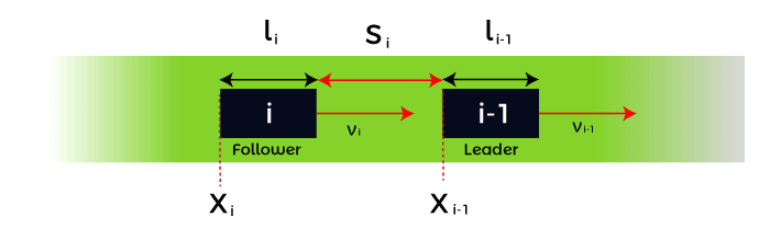
Every vehicle in microscopic models is numbered as i. The i-th vehicle follows the (i-1)-th vehicle. We will denote the position of the i-th vehicle along the road as xi, its speed as vi, and its length as li. And this is true for every vehicle. 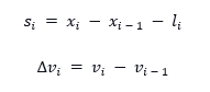
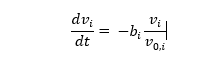
We will denote the bumper-to-bumper distance as si and the velocity difference between the i-th vehicle and the vehicle in front of it (vehicle number i-1) as ∆vi. Understanding the Intelligent Driver Model (IDM)In 2000, Treiber, Hennecke et Helbing developed a model called the Intelligent Driver Model. This model illustrates the acceleration of the i-th vehicle as a function of its variable and those of the vehicle in front of it. We can define the dynamics equation as shown below: 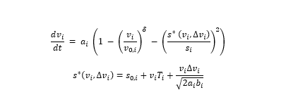
Since we have already seen the si, vi, and ∆vi, the other parameters are as follows: 1. s₀ᵢ: This parameter is the minimum desired distance between the vehicle i and i-1. 2. v₀ᵢ: This parameter is the maximum desired speed of the vehicle i. 3. δ: This parameter is the acceleration exponent, and it controls the "smoothness" of the acceleration. 4. Tᵢ: This parameter is the reaction time of the i-th vehicle's driver. 5. aᵢ: This parameter is the maximum acceleration for the vehicle i. 6. bᵢ: This parameter is the comfortable deceleration for the vehicle i. 7. s^*: This parameter is the desired distance between vehicle i and i-1. First, we will look at s^*, which is a distance comprised of three terms. 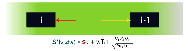
8. s₀ᵢ: This parameter, as said before, is the minimum desired distance. 9. vᵢTᵢ: This parameter is the reaction time safety distance. The distance the vehicle travels before the driver reacts (brakes). Since speed is distance over time, distance is speed times time. 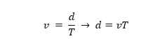
10. (vᵢ Δvᵢ)/√(2aᵢ bᵢ): This parameter is a more complicated term. It is a speed-difference-based safety distance. It signifies the distance it will take the vehicle to slow down (without hitting the vehicle in front), without breaking too much (the deceleration should be less than bᵢ). Understanding the working of the Intelligent Driver ModelWe can assume vehicles to be moving along a straight path and obey the following equation: 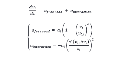
In order to get a better knowledge of the above equation, we can divide its terms in two. We have a free road acceleration and an interaction acceleration. 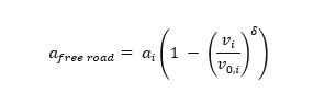
The free road acceleration is the acceleration on a free road: an empty road with no vehicles ahead. In case we plot the acceleration as a function of speed vi, we will get the following result: 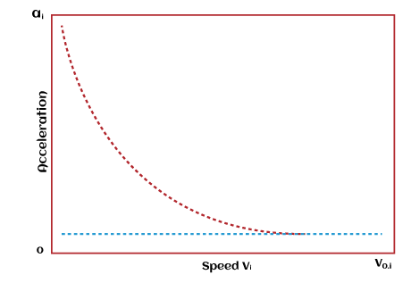
Image: Acceleration as a function of speed In the above graph, we notice that the acceleration is maximal when the vehicle is stationary (vi = 0). When the speed of the vehicle approaches the maximum speed v01, the acceleration turns zero. This statement implies that the acceleration of the free road will accelerate the vehicle to the maximum speed. In case we need to plot the v-a diagram from various values of δ, we will notice that it controls how quickly the driver decelerates when approaching the maximum speed, which in turn regulates the smoothness of the acceleration/deceleration. 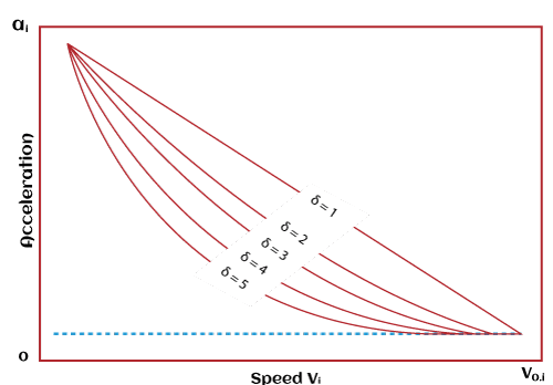
Image: Acceleration as a function of speed 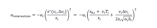
The interaction acceleration is connected to the interaction with the vehicle in front. We can understand its working in a better way by considering the following situations: On a free road (vi >> s^*): When the vehicle in front is far away, the distance si dominates the desired distance s*, and the interaction is almost 0. This indicates that we can govern the vehicle by free road acceleration. 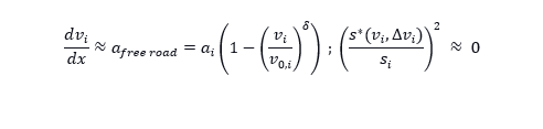
At high approach rates (∆vi): When the difference between the speed is high, the interaction acceleration attempts to compensate for that by braking or slowing down with the help of the (vi<vi)^2 term in the numerator; however, too hard. We can achieve this through the denominator 4bi si^2. 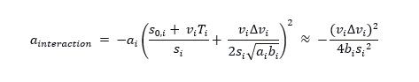
At small distance difference (?? << 1 and ∆?? = 0): The acceleration turns into a simple repulsive force. 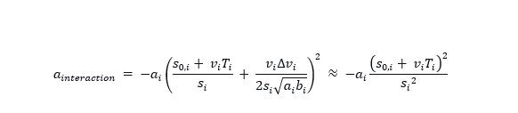
Understanding the Traffic Road Network Model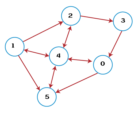
Image: Example of a directed graph Set: 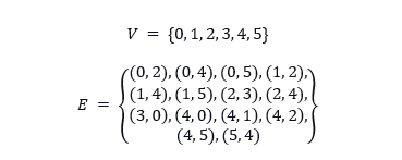
We have to model a network of roads. We can perform it with the help of a directed graph G = (V,E), where:
Every vehicle is about to have a path comprised of multiple roads (edges). We will apply the Intelligent Driver Model for vehicles on the same road (same edge). When a vehicle gets to the end of the road, we can remove it from that road and add it to its following road. We won't be keeping a set (array) of nodes in the simulation. However, every road is about to be defined by the values of its start and end nodes in an explicit way. Understanding the Stochastic Vehicle GeneratorWe have two options to include vehicles in the simulation: First Option: We can add every vehicle in a manual manner to the simulation by creating a new instance of Vehicle class and including it in the list of vehicles. Second Option: We can also use the stochastic way to add the vehicle per the pre-defined probabilities. In order to go with the second option, we need to define a stochastic vehicle generator. We can define a stochastic vehicle generator by two constraints:
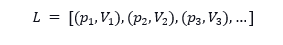
The stochastic vehicle generator generates the vehicle Vi with probability pi. Understanding the Traffic Light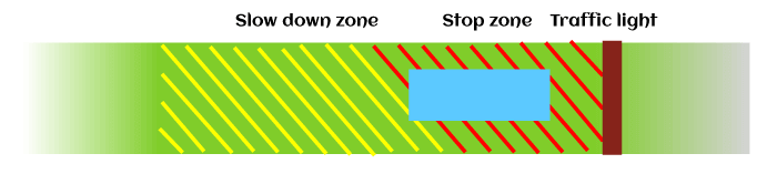
Traffic lights are placed at vertices and are characterized by two zones:
Project Code for Traffic Flow SimulationFor this project, we will adopt an object-oriented approach. Thus, every road and vehicle must be defined as a class. We will utilize the following initializing function frequently in various upcoming classes. This function will allow us to set the default configuration of the present class through a function set_default_config. It also expects a dictionary and sets every property in the dictionary as a property to the instance of the present class. In this manner, there is no need to worry about updating the __init__ functions of different classes or about alterations in the future. Let us consider the following snippet of code that illustrates the same: File: init.py Explanation: In the above snippet of code, we have defined the __init__() function that accepts the dictionary as config. Within this function, we have used the set_default_config() function in order to set the default configuration. We have then used the for-loop to iterate through the attributes and values present in the config dictionary and used the setattr() function to update the configuration for different classes. RoadWe will now create a Road class. Let us consider the following snippet of code demonstrating the same: File: road.py Explanation: In the above snippet of code, we have imported the distance function from the SciPy package and defined a class as Road. We have initialized some parameters as self, start, and end within this class using the __init__() function. We have then defined another function as initProperties() that calculates the left of the length of the road and the sine and cosine of its angle in order to draw it on the screen. SimulationWe will now create a Simulation class and add some methods to include roads to the simulation. Let us now consider the following snippet of code demonstrating the same: File: simulator.py Explanation: We have imported the Road class from the road.py file in the above snippet of code. We have then defined a class as Simulation. We have used the initializing function that we defined earlier within this class. We have then defined another function as set_default_config() and set some values of the attributes to default settings. We have then defined the function as createRoad() and createRoads() in order to create one and multiple roads. WindowWe will now display the Simulation on the screen in real-time. In order to perform this, we will utilize the pygame library and create a Window class that accepts a Simulation class as an argument. We will define different drawing functions that support drawing basic shapes. The loop method creates a pygame window and calls every frame the draw method and the loop argument. This will become helpful when the Simulation requires to be updated every frame. Let us consider the following snippet of code demonstrating the same: File: window.py Explanation: In the above snippet of code, we have imported the pygame library. We have then created a class as Window. We have initialized some parameters within this class and set the default configurations. We have then defined the loop function that displays a window visualizing the simulation and executes the loop function. We have then defined different functions like convert, inverseConvert, the_background, the_line, the_rect, the_box, the_circle, the_polygon, the_rotated_box, the_rotated_rect, drawAxes, drawGrid, drawRoads, drawStatus, and draw. We have saved the above files in a folder named trafficFlowSimulator. We will now create another python file as __init__.py and import the classes from the above files. File: __init__.py Explanation: In the above snippet of code, we have imported the classes from the python files we have created earlier. Let us now run a test code to see the output. File: testCase1.py Output: 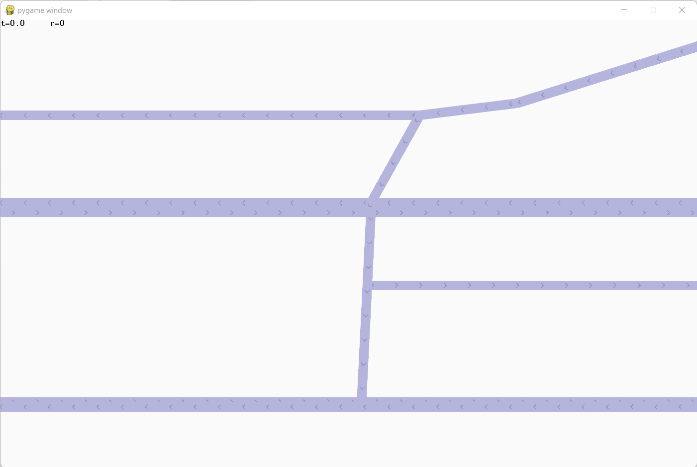
Explanation: In the above snippet of code, we have imported the classes from the trafficFlowSimulator. We have then created an object of the Simulator() class. We have then added a road using the createRoad() function that we created earlier. We have then added multiple roads using the createRoads() function. At last, we have started the simulation by creating an object of the Window() class and using the loop() function. VehiclesNow, we will add vehicles to the roads. We will be using the Taylor series in order to approximate the solution of the dynamic equations that we have discussed earlier in the modeling section of this tutorial. Taylor series expansion for an infinitely differential function f is: 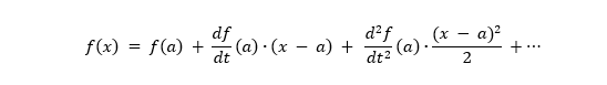
We will now substitute a by x and x by x + ∆x, we will get: 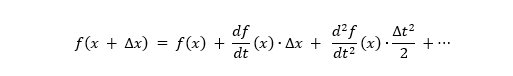
We will now replace f by the position x: 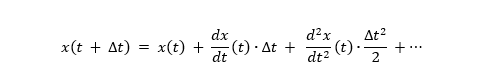
As a precision, we will stop at order 2 for position as acceleration is the highest-order derivative. We get equation (2): 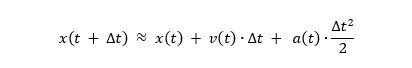
Equation (2) For speed, we will substitute x by v: 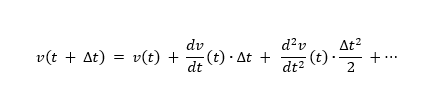
We will stop at order 1, as the highest-order derivative we have is acceleration (order 1 for speed). Equation (2): 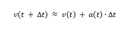
Equation (1) In every iteration (or frame), once we calculate the acceleration with the help of the IDM formula, we will update the position and speed using these two equations: Equation (1) 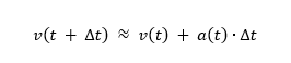
Equation (2) 
Let us consider the following snippet of code demonstrating the same: File: numericalApprx.py Explanation: Since the above snippet of code is only an approximation, the speed can sometimes become negative (however, the model does not permit that). An instability arises when the speed is negative, and the position and speed diverge into negative infinity. We can overcome this problem by predicting a negative speed and setting it equal to zero, and working out way from there: 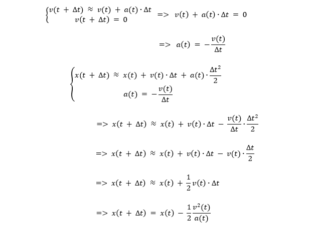
Let us consider the following snippet of code demonstrating the same: File: negativeSpeed.py Explanation: In the above snippet of code, we have used the if-else conditional statement to check if the speed is negative. In order to calculate the IDM acceleration, we will denote the lead vehicle as leadVehicle and calculate the interaction term (denoted alpha) when leadVehicle is not None. Let us consider the following snippet of code demonstrating the same: File: leadVehicle.py Explanation: In the above snippet of code, we have initialized the value of alpha as zero. We have then used the if conditional statement to calculate the del_x and del_v and alpha value. In case the vehicle is stopped (for example, at a traffic light), we will utilize the damping equation. After then, we will combine everything in an update method within a Vehicle class. Let us consider the following snippet of code demonstrating the same: File: vehicle.py Explanation: In the above snippet of code, we have imported the required module and defined a class as Vehicle. We have used the __init__() function and set the default configurations within this class. We have then defined the initProperty() function along with the update() function that updates the position, the velocity, and the acceleration. We have also defined functions to stop, unstop, slow down and increase the velocity of a vehicle. In the Road class, we will include a deque (also known as a double-ended queue) in order to keep track of vehicles. A data structure like a queue is better in storing vehicles as the first Vehicle in the queue is the farthest one down the road and is the first one that we can remove from the queue. We can remove the first data element from a deque using the self.vehicles.popleft(). We will include an update method in the Road class. Let us consider the following snippet of code to understand the same: File: road.py Explanation: In the above snippet of code, we have defined a function as an update for the Road class. Within this function, we have assigned the length of the vehicles in deque to a variable num and used the if condition to check if it is greater than zero and update the first vehicle. We have then used the for-loop ranging from 1 to num and updated the rest of the vehicles in the deque. Now let us add an update method to the Simulation class as well. Here is the following snippet of code demonstrating the same: File: simulation.py Explanation: In the above snippet of code, we have defined an update() function in the Simulation class. Within this function, we have updated every road. We have then checked the roads for out-of-bounds vehicles and performed the operations accordingly. Now, let's get back to the Window class and add a run method in order to update the simulation in real-time: File: window.py Explanation: In the above snippet of code, we have defined a run method that updates the simulation in every loop. For now, we will include vehicles manually: File: testCase2.py Output: 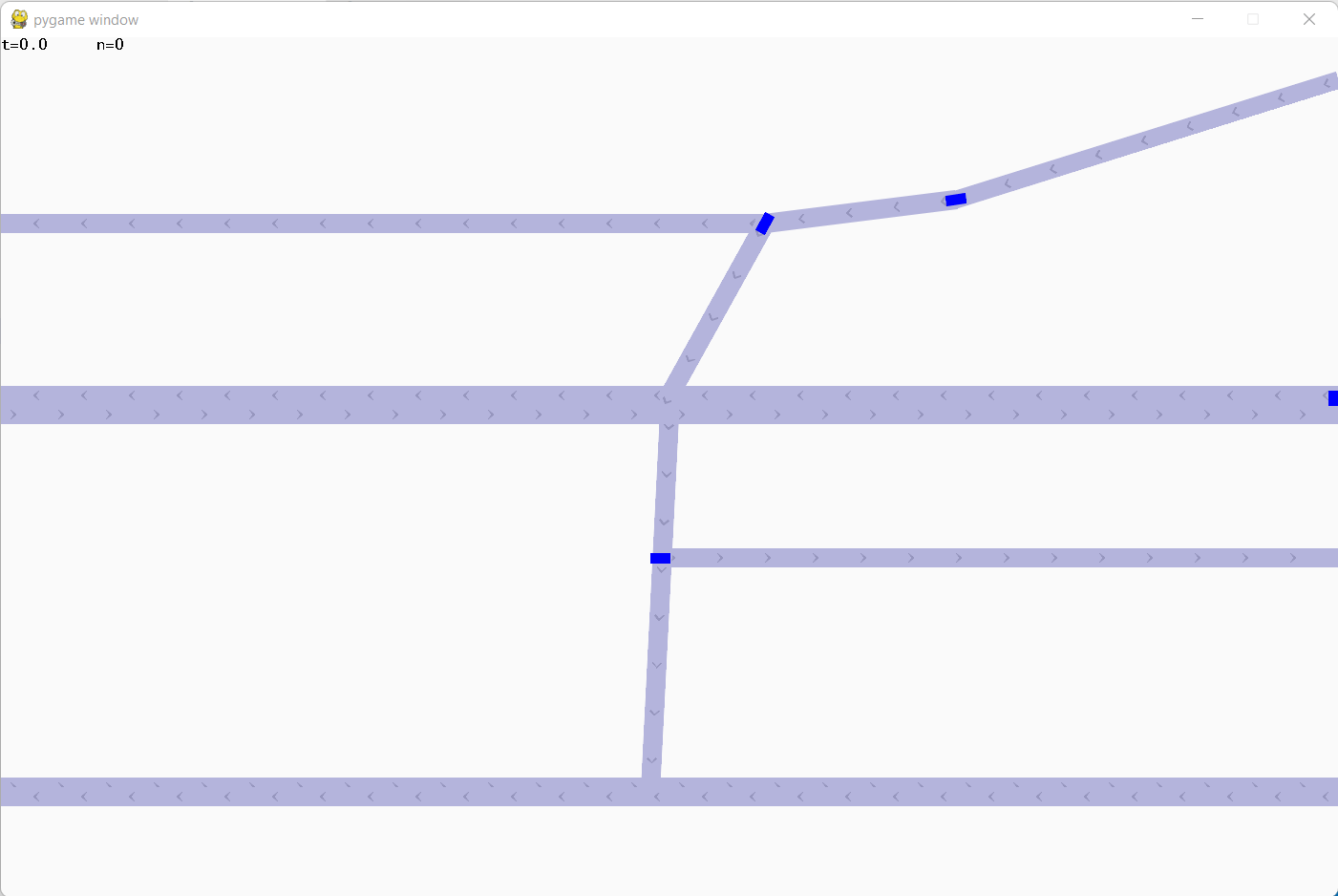
Explanation: In the above snippet of code, we manually added the vehicles to the roads we created earlier. We have used the append() function to insert vehicles on different roads. Vehicle GeneratorsFile: vehicleGenerator.py Explanation: In the above snippet of code, we have imported the Vehicle class from the vehicle.py file and the randint function from the numpy library. We have then created a class as VehicleGenerators and defined the __init__ function setting the default configuration and initProperties. We have then included the functions like generateVehicle and update to return a random vehicle from self.vehicles with random proportions and add vehicles. A VehicleGenerators class has an array of tuples (odds, vehicle). The first data element of the tuple is the weight (not probability) of the vehicle generation in the same tuple. We have used weights as they are convenient to work with since we can utilize integers. For instance, if we have three vehicles with weights 3, 1, 2. This corresponds to 3/6, 1/6, 2/6 with 6 (= 3 + 1 + 2). We can utilize the following algorithm in order to implement this:
Suppose that we have weights as W1, W2, W3. The following algorithm will allow us to allocate numbers between 1 and W1 to the first vehicle, numbers between W1 and W1 + W2 to the second vehicle, and numbers between W1 + W2 + W3 to the third vehicle. File: vehicleGenerator.py Explanation: In the above snippet of code, we have defined a function as generateVehicle(). We have calculated the sum of the pair in the self.vehicles within this function and returned a random vehicle with random proportions. We have included a property known as lastAddedTime so that whenever we add a vehicle, the current time will be updated every time the generator performs the function. When the time duration between the current time and lastAddedTime is greater than the period of vehicle generation, a vehicle is included. The period of adding vehicles is 60/vehicleRate because vehicleRate is in vehicles per minute, and 60 is 1 minute or 60 seconds. We will also check if the road has any space to add the upcoming vehicle. We perform this operation by checking the distance between the last vehicle on the road and the sum of the length and safety distance of the upcoming vehicle. Let us consider the following snippet of code demonstrating the same: File: vehicleGenerator.py Explanation: In the above snippet of code, we have defined an update() function in order to add vehicles to the simulation. We have used the if conditional statement to check whether the time elapsed after the addition of the last vehicle is greater than the vehicle period and generating a vehicle for the same. We have also checked if any space is present for the generated vehicle and added it. At last, we have reset the time of the last addition and upcoming vehicle. Finally, we should update vehicle generators by calling the update method from the Simulation class. Let us consider the following snippet of code to understand the same: File: testCase3.py Output: 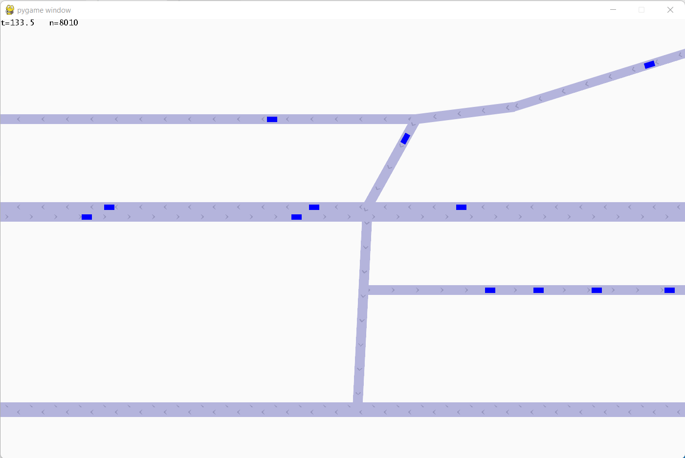
Explanation: In the above snippet of code, we have initialized the createGen function of the Simulation class and provided the required values to the parameters like vehicleRate and vehicles. We have also specified the paths for the vehicles and executed the program. Traffic LightsLet us now add the traffic light and its properties to the simulation. The default properties for a traffic signal are as follows: File: trafficLight.py Explanation: In the above snippet of code, we have defined a class as TrafficSignal. We have used the __init__() function to initialize some variables and functions within this class. We have then defined another function to set the default configuration. The self.cycle variable is an array of tuples consisting of the states (for example, True symbolizes green and False symbolizes red) for every road set in self.roads. In the default configuration, the data element (False, True) indicates the first set of roads is read and the second one is green (True, False) is the opposite. We will use this approach as it is easily scalable. We create traffic lights involving more than two roads, traffic lights with distinct signals for right and left turns, or even synchronized traffic signals across different intersections. The update function of a traffic signal will be customizable. The default behaviour of this function will be symmetric fixed-time cycling. File: trafficLight.py Explanation: In the above snippet of code, we have defined the initProperties() function. We have then used the for-loop iterating through each road in the array and setting all the signals within this function. We have then defined a function to return the current cycle index. We have then defined an update function where we have gone through all cycles and repeat. Now we will include the following methods in the Road class. File: road.py Explanation: In the above snippet of code, we have defined the functions to set the Traffic signal and its state for each cycle. We will now add the following snippet of code in the update function of the Road class. File: road.py Explanation: In the above snippet of code, we have checked for the traffic signal and perform the specific set of tasks for specific signal. We will now check for the state of the traffic light in the update method of the Simulation class: File: simulator.py Explanation: In the above snippet of code, we used the for-loop to iterate through each signal in the trafficSignals array and update them. Here is an output for the same: Output: 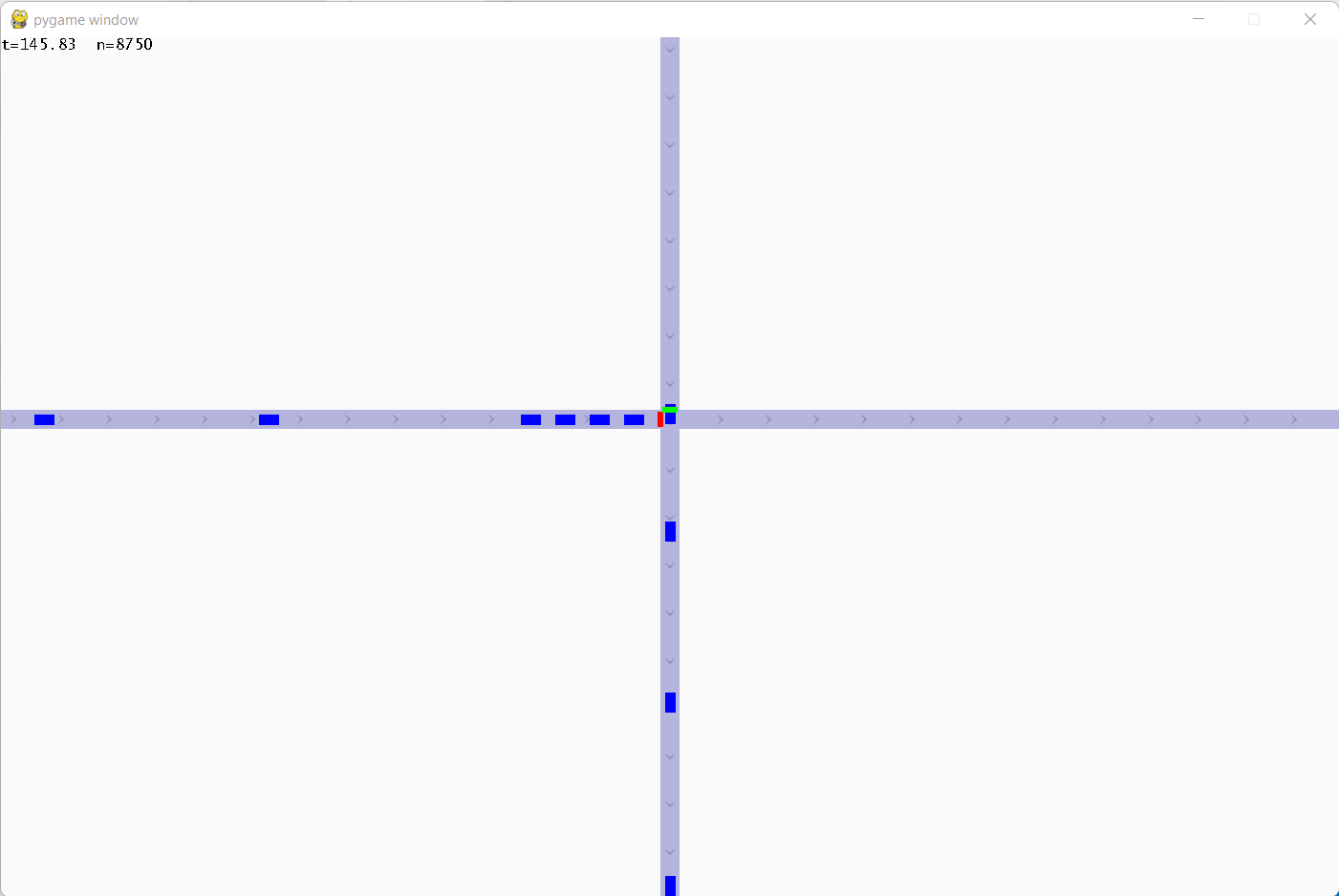
CurvesThe roads in the real world have curves. Since we can, technically, create curves in this traffic flow simulation by hand-writing the coordinates of a lot of roads to estimate a curve, we can perform the same thing in a procedural way. We will be using Bezier curves for this. We will create a curve.py file consisting of the functions helping in creating curves and referencing them by their road indices. Let us consider the following snippet of code demonstrating the same: File: curve.py Explanation: In the above snippet of code, we have defined a function as curvePoints(). We have then checked if the curve was a straight line or not and performed the operations accordingly. We have then defined another function as curveRoad() that returns the curved path. Let us now test the above code for better illustration. File: testCase3.py Explanation: In the above snippet of code, we have imported the folder containing classes we created earlier. We have then created an instance of the Simulator() class. We have then added multiple roads. We have also included the curveRoad() function to create a curve road. We have then added vehicles to the simulation and executed the program. Output: 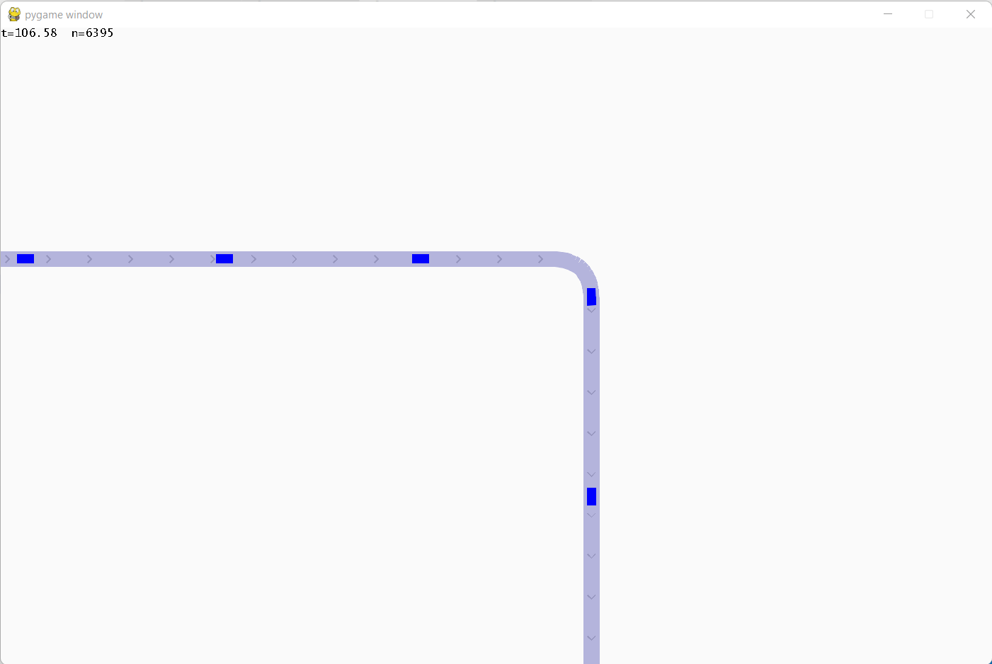
LimitationsWhile we can modify the Simulation class to store data related to the simulation that we can utilize later, it would be better if gathering data was more streamlined. This simulation is still lacking a lot. The curves implementation is bad and inefficient and causes issues with interaction between vehicles and traffic signals. While some may be concerned about the Intelligent Driver Model is a bit overkill, it is significant to have a model that can replicate real-world phenomena such as traffic waves (also known as ghost traffic snakes) and the effects of the driver reaction time. For the same reason, we opted to utilize the Intelligent Driver Model. However, in order to create a simulation where precision and extreme realism are not significant, like in video games, we can substitute IDM with a simpler logic-based model. Depending completely on simulation-based data increases the risk of over-fitting. The ML model could be optimizing for treats available in the simulation and absent in the real world. ConclusionSimulation is one of the significant segments of data science and machine learning. Sometimes, collecting data from the real world is either not possible or costly. And data generation supports building huge datasets at a somewhat better price. Simulation can also support filling the gaps in real-world data. On a few occasions, real-world datasets lack edge cases that may be critical to the developed model. |

 For Videos Join Our Youtube Channel: Join Now
Feedback
- Send your Feedback to [email protected]
Help Others, Please Share


