| |
Python Tutorial
Python OOPs
Python MySQL
Python MongoDB
Python SQLite
Python Questions
Plotly
Python Tkinter (GUI)
Python Web Blocker
Python MCQ
Related Tutorials
Python Programs

Maxwell Distribution in Statistics using PythonThe scipy.stats.maxwell(), known as the Pareto of the Second Kind, defines the Maxwell continuous random variable. It is an instance of the rv_continuous class inherited from the generic methods. It completes the techniques by adding details specific to this distribution. The Parameters included in the scipy.stats.maxwell() are:
By default, it is 'mv' (mean and variance)
The scipy library in Python offers different packages for calculating the Maxwell Distribution in Statistics named scipy.stats. This package provides a module named Maxwell which can be used for the Maxwell Distribution. The probability density function for Maxwell distribution
The probability density function defined is the standardized form. We use the loc and scale parameters to shift and scale the distribution. The shifting of the location does not make it a noncentral distribution. maxwell.pdf(x, loc, scale) is exactly equal to maxwell.pdf(y) / scale with y = (x - loc) / scale. Importing Maxwell library in PythonLet's understand the concept of the Maxwell distribution of Statistics using Python. Program 1: A program to create Maxwell Continuous Random Variable Code: Output: Random Variable : <scipy.stats._distn_infrastructure.rv_continuous_frozen object at 0x000001E2E634D690> Explanation: In this, we have imported the Maxwell module. Then we assign two random variables, then using the maxwell() function, we will print the continuous Maxwell distribution of the random variables. Program 2: A program to create Maxwell Continuous Variates and Probability Distribution. Code: Output: Random Variates : 10.539285144564246 The Probability Distribution : [0.00000000e+000 0.00000000e+000 0.00000000e+000 0.00000000e+000 0.00000000e+000 0.00000000e+000 0.00000000e+000 0.00000000e+000 0.00000000e+000 0.00000000e+000 0.00000000e+000 0.00000000e+000 0.00000000e+000 0.00000000e+000 0.00000000e+000 0.00000000e+000 0.00000000e+000 1.72263302e-315 6.11825318e-286 2.47898060e-260 5.36942377e-238 2.12617884e-218 4.13678696e-201 8.82118836e-186 3.97454825e-172 6.50201331e-160 6.05449810e-149 4.67357077e-139 4.10318936e-130 5.35464112e-122 1.30425958e-114 7.20412955e-108 1.06667729e-101 4.89121972e-096 7.87177281e-091 4.95770326e-086 1.34380703e-081 1.70387824e-077 1.08747806e-073 3.72710529e-070 7.26359302e-067 8.46886995e-064 6.18063913e-061 2.93969655e-058 9.44744338e-056 2.11900932e-053 3.41508081e-051 4.05984061e-049 3.64536233e-047 2.52580579e-045 1.37695729e-043 6.01120706e-042 2.13546523e-040 6.26418545e-039 1.53771874e-037 3.19765978e-036 5.69622937e-035 8.78208419e-034 1.18291931e-032 1.40418650e-031 1.48072561e-030 1.39734406e-029 1.18813409e-028 9.15994482e-028 6.44043041e-027 4.15217863e-026 2.46690167e-025 1.35694853e-024 6.94049040e-024 3.31422417e-023 1.48309519e-022 6.24126284e-022 2.47806223e-021 9.31140578e-021 3.32064814e-020 1.12693035e-019 3.64860395e-019 1.12962130e-018 3.35176698e-018 9.55101796e-018 2.61882508e-017 6.92213756e-017 1.76685183e-016 4.36206431e-016 1.04323334e-015 2.42044968e-015 5.45542325e-015 1.19601990e-014 2.55361264e-014 5.31592344e-014 1.08014757e-013 2.14445337e-013 4.16393728e-013 7.91495858e-013 1.47411758e-012 2.69226174e-012 4.82556855e-012] Explanation: In this, we have given a numpy array and will print the random variates and the probability distribution of the numpy array. Program 3: A program to show the graphical representation of the Maxwell Probability Distribution function. Code: Output: Distribution : [0. 0.10204082 0.20408163 0.30612245 0.40816327 0.51020408 0.6122449 0.71428571 0.81632653 0.91836735 1.02040816 1.12244898 1.2244898 1.32653061 1.42857143 1.53061224 1.63265306 1.73469388 1.83673469 1.93877551 2.04081633 2.14285714 2.24489796 2.34693878 2.44897959 2.55102041 2.65306122 2.75510204 2.85714286 2.95918367 3.06122449 3.16326531 3.26530612 3.36734694 3.46938776 3.57142857 3.67346939 3.7755102 3.87755102 3.97959184 4.08163265 4.18367347 4.28571429 4.3877551 4.48979592 4.59183673 4.69387755 4.79591837 4.89795918 5. ] 
Explanation: We have printed the distribution of the numpy array, and then using matplotlib, we have printed a graph of the Maxwell Distribution using the Probability Density function. Program 4: A program to graphically represent varying positional arguments in the Maxwell Probability Distribution Function. Code: Output: [ 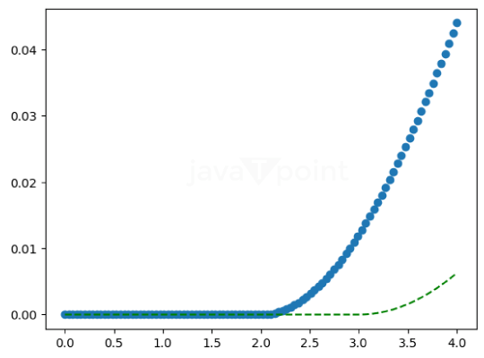
Explanation: We made a numpy array with linear, equal spaces, then plotted a graph with two different Probability Density Functions. |
 For Videos Join Our Youtube Channel: Join Now
Feedback
- Send your Feedback to [email protected]
Help Others, Please Share


