Unemployment Data Analysis using Python

How to calculate unemployment rate?

The number of unemployed persons as a proportion of the total labor force is used to calculate the Unemployment rate, which is used to assess Unemployment. The Unemployment rate has significantly increased during COVID-29, making its analysis a worthwhile data science research. We'll walk you through the Python source code of Unemployment analysis in this tutorial.

Introduction: Since 2020, several organizations have kept official records on Unemployment in the United States. The U.S. Department of Labor's Bureau of Labour Statistics (BLS) releases information regarding the overall number of employed and jobless individuals in the U.S. for the previous month and various other statistics early each month. The unemployment rate is determined by multiplying the civilian labor force by the number of jobless persons. To qualify as "unemployed," a person must be under sixteen years old, have not had a part-time or full-time job for at least four weeks, and have been actively seeking employment.

Our group decided to examine U.S. Unemployment statistics, emphasizing the years 2000 through 2023. Our stringing was to forecast the jobless rate for the next year, 2023, using data from this period. We intend to forecast discrete numbers for each month in 2023 because the BLS only provides data on the jobless rate in discrete monthly increments. To determine how the various variables affect the rate, we want to put our data science expertise to the test.

Data Exploration and Analysis

We gathered data sets from the Bureau of Labour Statistics website (BLS), a federal agency that offers information on the U.S. labor market's activity, labor conditions, price fluctuations, and productivity. Additionally, we looked at data from one of the most dependable sources of financial information in the country, The Federal Reserve Bank of St. Louis' Federal Reserve Financial Database [https://fred.stlouisfed.org/]. The 20+ years of data in the CSV files we acquired (2000-2023) provide a good historical perspective that may be used to forecast future events. Data on educational attainment, race, and gender are included in some of the data fields we scrutinize.

We utilized an API key to scrape data from the website for the data discovery phase. Using the reduce() technique, we chose a few reports relevant to the U.S. jobless rate, mapped them into a DataFrame, and then saved the outcomes as a CSV file. Then used, Python to remove redundant or empty rows and columns from the data and consolidate similar categories into a single CSV file (for example, different CSV files for Male and Female information combined into gender.csv).

We established an AWS RDS cloud database and connected using a connection string. This was done after all the CSVs had been filtered and cleaned only to include relevant data.

Dataset

Importing the appropriate Python modules and using the dataset will allow us to begin Unemployment Data Analysis using Python

Main table (for reference only):

Machine Learning Models

Our machine learning models are used to implement the project's analysis phase. Rather than being predominantly categorized, our data are continuous. So instead of making a binary prediction, we'll make a numerical one. What the Unemployment rate will be by the end of December 2023 or the next month is the forecast we are attempting to make.

K-Nearest Neighbor Model

The K-Nearest Neighbour (KNN) method is one of the models created using machine learning that we will be putting into practice. KNN can be applied to classification or linear regression. We will divide the extra data into training and testing sets for our research, including consumer pricing for meat and job vacancies for various industries retrieved during the API request.

Observation:

• The rate of Unemployment will be utilized as the aim (Y), while the data on job vacancies and meat costs will be used as the characteristics (X).
• We determined that it would be preferable to utilize only two years' worth of collected information (The year 2002) and attempt to forecast the next year's worth of info (The year 2002) to verify that the predicted data is correct and a good match.
• The outcomes will then be represented as a graph. However, before doing this, we tested it using the API to retrieve different data types to check whether it would function. Please use the ML-KNN.py file as a guide.
• A graph appeared to have been produced, and the code worked. For the outcomes, see below. Next, we want to update the code to work with the relevant datasets indicated before.

Support Vector Regression Model

The SVR model is A supervised learning model frequently used to forecast discrete values. Since our project's stringing was to forecast discrete jobless rate figures for each month in 2023, this would help us achieve it.

Observation:

• The first dataset we provided the model appeared to function and generate an accuracy score. However, subsequent attempts to change the dataset ultimately resulted in us breaking the code.
• We could not proceed with the real rate prediction because of the faults we discovered in the model's preliminary accuracy prediction phase.
• Additionally, due to our little time, we needed more time to plot the findings as required.
• Consequently, this model proved to be unsuitable for the project. If we had more time to fix the programming issues, this approach would eventually prove trustworthy and helpful.

Auto-Regressive Integrated Moving Average Model

As another time series forecasting model, we investigate the AutoRegressive Integral Moving Average (ARIMA) machine learning model. A common ML technique for estimating the future values that a series will take is forecasting. A time series might be annually (for example, an annual budget), quarterly (for example, costs), monthly (for example, air traffic), weekly, daily, hourly (for example, stock prices), minutes (for example, incoming calls at a call center), or even seconds (for example, web traffic). Since jobless rate data is normally provided on a monthly or annual basis and since our goal is to forecast potential values for the rate of jobless at either the end of the year in December of that year or even at the end of the following month, this suits our research. To forecast the U.S. overall jobless rate and each factor by December 2023, we want to apply a Time Series model to quantify potential joblessness rates using a single dataset CSV each time.

Observation:

• The ARIMA test's mathematical underpinnings are quite complex, and the model itself has several variants, even though they all operate on the same principles. On datasets with stationarity (no trends), ARIMA performs best.
• If a dataset is not stationary, a technique called "differencing" can be used to make it stationary; fortunately, our datasets were proved stationary by executing a few useful lines of Python script.
• Without getting into great detail about the operation of the ARIMA model, one of the most important things to remember is the optimal order in which to apply it, which is determined by the Akaike Information Criterion, or AIC, score with the lowest value.
• The order comprises three numerical numbers in the format (p,d,q), where p stands for the model's lag observations' number, d for the number of times raw data is differenced, and q for the moving average window's size. We utilized several lines of template code and a helpful built-in Python tool to assist us in getting this order for our representation, which turns out to be (0,2,0).
• We tried several approaches to the ARIMA test, but we needed a trustworthy answer. Although we are confident that there are answers, each of the tried alternatives had unique problems along the route that we needed help to resolve in the allotted time.
• The overall_monthly.csv dataset of the national jobless rate from 2000 to 2023 was used for all three experiments. First, we wanted to determine the expected national rate for each of the 22 months 2023.
• If the test was successful, we planned to repeat it for the other categories. However, given that we had problems even with the initial categorical dataset, we concluded that these problems would continue regardless of the category dataset chosen.
• We tried several approaches to the ARIMA test, but none of them gave us a trustworthy answer. Although we are confident that there are answers, each of the tried alternatives had unique problems along the route that we needed help to resolve in the allotted time. The overall_monthly.csv dataset of the national Unemployment rate from 2000 to 2023 was used for all three experiments.

First, we wanted to determine the expected national rate for each of the 22 months 2023. If the test was successful, we planned to repeat it for the other categories. However, given that we had problems even with the initial categorical dataset, we concluded that these problems would continue regardless of the category dataset chosen.

Installation

• You must install Python 5 and the following Python libraries to use this project: Plotly, Pandas, Matplotlib, and NumPy.
• The following commands can be used to install these libraries: install pandas using pip matplotlib, and numpy is installed using pip. Install pip seaborn Plotly installation
• Alternatively, install the libraries using the pip install -r requirements.txt command from the project directory.

Usage

Use this project by doing the following:

1. Clone the project repository to your computer locally in step 2.
2. Launch a command prompt or terminal to the project directory.
3. Use the following command to launch the script jobless_analysis.py:
4. Python file called Jobless_analysis_with_Python.py
5. The script will request the name of the nation whose jobless statistics you wish to examine. Press Enter after entering the country's name.
6. To better understand the patterns and developments in the data, the script will read Unemployment data from a spreadsheet located in the data directory and produce visualizations. The output directory will house the visualizations.

Unemployment Analysis with Python Source Code

I will use a dataset of unemployment in India to analyze unemployment, as the unemployment rate is determined based on a specific location. The dataset I'm utilizing here includes information on India's unemployment rate from 2003 to 2029. Therefore, let's begin the work of analyzing Unemployment by importing the required Python modules and the dataset:

ANALYZING DATASET

Reading the Data

Source Code Snippet

Output:

Source Code Snippet

Output:

Source Code Snippet

Output:

Source Code Snippet

Output:

Region                                       string
 Date                                        string
 Frequency                                   string
 Estimate Jobless Rate (%)            float64
 Estimate Employed                         float64
 Estimate Labour Participation Rate (%)    float64
Area                                         string
dtype: string

Source Code Snippet

Output:

DATA PROCESSING

The data entered into the computer in the preceding phase is actually processed for interpretation at this stage. The process itself could differ slightly depending on the source of the data being processed (data lakes, social media platforms, connected devices, etc.) and the purpose for which it is used (studying advertising patterns, medical diagnosis from associated devices, deciding customer needs, etc.). Processing is carried out using machine learning algorithms.

Source Code Snippet

Output:

Region                                      28
 Date                                       28
 Frequency                                  28
 Estimate Jobless Rate (%)            28
 Estimate Employed                         28
 Estimate Labour Participation Rate (%)    28
Area                                        28
dtype: int64

Source Code Snippet

Output:

(968, 9)

Source Code Snippet

Output:

Region                                      0
 Date                                       0
 Frequency                                  0
 Estimate Jobless Rate (%)            0
 Estimate Employed                         0
 Estimate Labour Participation Rate (%)    0
Area                                        0
dtype: int64

Source Code Snippet

Output:

(940, 9)

Let's check to see whether this dataset has any missing values:

Source Code Snippet2

Output:

Region                                      0
Date                                        0
 Frequency                                  0
 Estimate Jobless Rate (%)            0
 Estimate Employed                         0
 Estimate Labour Participation Rate (%)    0
Region.2                                    0
longitude                                   0
latitude                                    0
dtype: int64

After looking into the missing values, I discovered those column names are incorrect. In order to make this data easier to grasp, I will change all the columns as follows:

Source Code Snippet

Let's now examine the relationship between the characteristics of this dataset:

Source Code Snippet

Output:

Let's now analyze the unemployment rate by visualizing the data. I'll start by looking at the estimated number of employees by India's various regions.

Source Code Snippet

Output: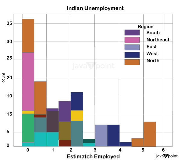

Let's examine the unemployment rate in India's various areas.

Source Code Snippet

Output: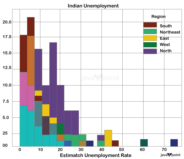

Create a dashboard now to examine the unemployment rate in each Indian state by area. I'll employ a sunburst layout in this.

Source Code Snippet

Output: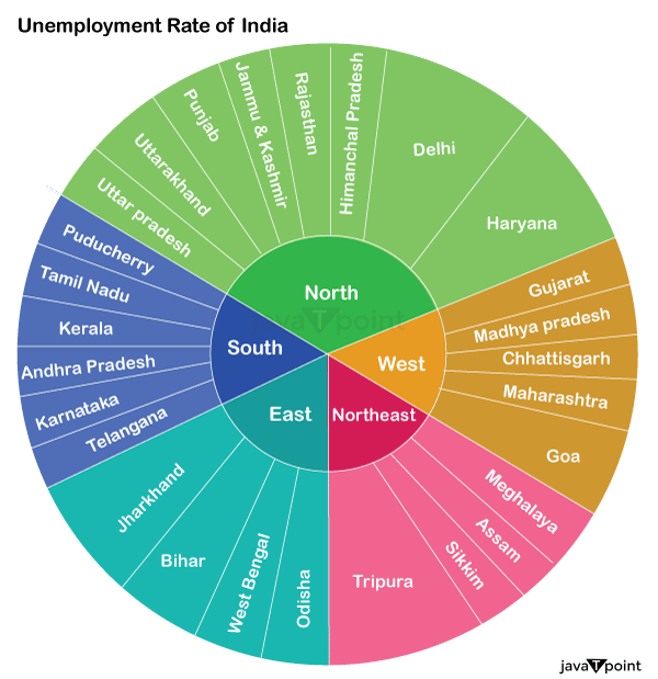

Summary

So here is how you can use the Python language to analyze the jobless rate. The number of unemployed persons as a proportion of the total labor force is used to calculate the Unemployment rate, which is used to assess Unemployment. I hope you enjoyed reading this tutorial on Python-based Unemployment rate analysis.