| |

Sklearn ClusteringOne method for learning about anything, like music, is to look for significant groupings or collections. While our friends may arrange music by decade, we may arrange music by genre, and our choice of groups aids in understanding the distinct elements. What is Clustering?One of the unsupervised machine learning techniques, called clustering, is a means to find connections and patterns among datasets. The dataset samples are then organized into classes based on characteristics that have a lot of similarities. Because it guarantees the natural clustering of the available unlabelled data, clustering is essential. It is defined as an algorithm for categorizing data points into different classes according to their similarity. The objects that might be comparable are maintained in a cluster that bears little to no resemblance to another cluster. This is done by finding similar trends in an un-labelled dataset, such as the activity, size, colour, and shape, and then classifying the data based on whether or not such trends are present. Because the algorithm is an unsupervised learning technique, it operates on an un-labelled dataset and gets no supervision. Un-labelled data can be clustered using the sklearn.cluster method in the Scikit-learn module of Python. Now that we are familiar with clustering, let's investigate the various clustering methods available in SkLearn. Clustering Methods in Scikit-learn of Python
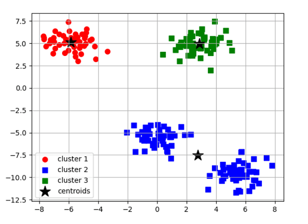
KMeansThe centroids of the clusters of different data classes are calculated by this algorithm, which then identifies the ideal centroid through iteration. It assumes there are previously known clusters for the given dataset because it needs the number of clusters as its parameter. The fundamental idea behind this clustering method is to cluster the provided data by splitting samples into n number of groups with identical variances while reducing the inertia constraint. The number of clusters is represented by k. Python Scikit-learn has sklearn.cluster.KMeans clustering to perform the KMeans clustering. The sample weight argument enables sklearn.cluster to compute the cluster centres and inertia value. KMeans module to give some samples additional weight. Algorithm of K-Means ClusteringA set of N number of samples is divided into K number of disjoint clusters via the k-means clustering algorithm, and each cluster's mean is used to characterize its samples. Although they share a similar space, the means are often referred to as the cluster's "centroids". The centroids are usually not the points from the independent feature X. To minimize the sum of squares criterion within the cluster, or inertia, is the goal of the Kmeans clustering method. The algorithm of the k-means clustering method, which the four significant steps can sum up, can be used to cluster the samples into different classes depending on how related their features are. Select k number of centroids randomly from the sample locations to serve as the first cluster centres. Place each sample point next to its closest centroid. Position the centroids in the middle of the sample points given to the clusters. Repeat steps 2 and 3 to attain a tolerance level defined by the user, the maximum number of iterations, or until no changes to the cluster classes are observed. Python Scikit-Learn Clustering KMeansParameters n_clusters (int, default = 8):- This number represents the number of centroids to create and the number of clusters to construct. Init ({'k-means++', 'random'}, array-like having shape (n_clusters, n_features), default = 'k-means++'):- The initialization method. To hasten convergence, "k-means++" intelligently chooses the starting cluster centres for k-mean clustering. "random" randomly select the number of clusters observations (rows) for the starting centroids from the dataset. n_init (int, default = 10):- The number of iterations the k-means clustering algorithm will undergo using various centroid seeds. The end scores will be the inertia-minimized best result of n_init successive cycles. max_iter (int, default = 300):- This specifies the maximum number of k-means clustering algorithm iterations in a single run. tol (float, default = 1e-4):- Convergence is defined as the distance between the cluster centres of two successive iterations with a proportional tolerance with respect to the Frobenius norm. verbose (int, default = 0):- Mode of verbosity. random_state (int, RandomState instance or None, default = None):- This parameter determines how the centroid initialization random sample is generated. Make the randomization deterministic by using an int. copy_x (bool, default = True):- When calculating distances beforehand, it is more quantitatively precise to centre the data first. The initial data is not changed if x_copy is set to True (the default value). If False, the initial data is changed and restored before the method exits. algorithm ({"lloyd", "elkan", "auto", "full"}, default = "lloyd"):- Specifies the algorithm of the K-means clustering method to use. Code Output: 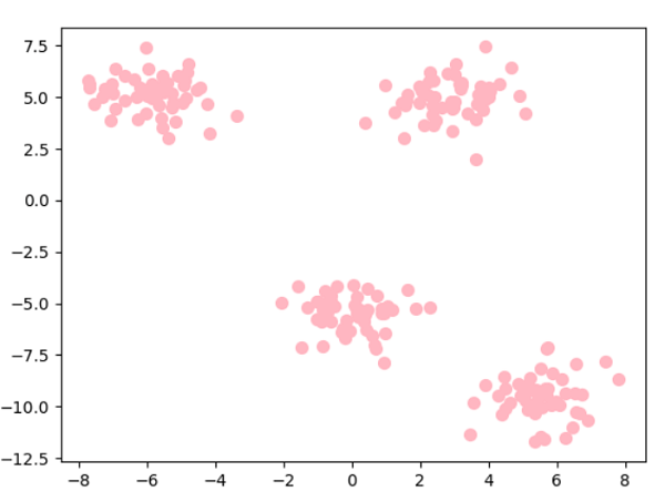
The Elbow MethodEven though k-means performed well on our test dataset, it is crucial to stress that one of its limitations is that we must first define k, the number of clusters, before we can determine what the ideal k is. In real-world situations, the number of clusters to select might not always be evident, mainly if we deal with a dataset with high dimensions that cannot be seen. The elbow technique is a helpful graphical tool to determine the ideal number of clusters, k, for a specific activity. We can infer that the within-cluster SSE ( or distortion) will decrease as k grows. This is so that the data will be nearer their designated centroids. Code Output: 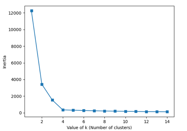
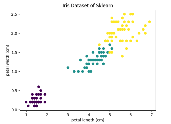
Hierarchical ClusteringForming clusters from data using a top-down or bottom-up strategy is known as hierarchical clustering. Either it begins with a solitary cluster made up of all the samples included in the dataset and then divides that cluster into additional clusters, or it begins with several clusters made up of all the samples included in the dataset and then combines the samples according to certain metrics to generate clusters with even more measurements. As hierarchical clustering advances, the results can be seen as a dendrogram. Tying "depth" to a threshold aids us in determining how deeply we want to cluster (when to stop). It has 2 types: Agglomerative Clustering (bottom-up strategy): Starting with individual samples of the dataset and their clusters, we continuously combine these randomly created clusters into more prominent clusters based on a criterion until only one cluster is left at the end of the process. Divisive Clustering (top-down strategy): In this approach, we begin with the entire dataset at a time combined as one solitary cluster and continue to break this cluster down into multiple smaller clusters until each cluster contains just one sample. Single Linkage: Through this linkage method, we combine the two clusters with the most comparable two members, using pairs of elements from each cluster that are the most similar to one another. Complete Linkage: Through this linkage method, we select the most different samples from each cluster and combine them into the two clusters with the smallest dissimilarity distance. Average Linkage: In this linkage approach, we use average distance to couple the most comparable samples from every cluster and combine the two clusters containing the most similar members to form a new group. Ward: This approach reduces the value of the sum of the squared distances calculated for all the cluster pairs. Although the method is hierarchical, the idea is identical to KMeans. Be aware that we base our comparison of similarity on distance, which is often euclidean distance. Parametersn_clusters (int or None, default = 2):- The number of clusters to be generated by the algorithm. If the distance threshold parameter is not None, it must be None. affinity (str or callable, default = 'euclidean'):- This parameter suggests the metric employed in the linkage computation. L1, L2, Euclidean, Cosine, Manhattan, or Precomputed are all possible options. Only "euclidean" is acceptable if the linkage method is "ward." If "precomputed", the fit technique requires a proximity matrix as input rather than a similarity matrix). memory (str or an object having joblib.Memory interface, default = None):- It is used to store the results of the tree calculation. Caching is not carried out by default. The path to access the cache directory is specified if a string is provided. connectivity (array-like or a callable object, default = None):- This parameter takes the connectivity matrix. compute_full_tree ('auto' or bool, default = 'auto'):- At n_clusters, the algorithm stops the tree's construction. linkage ({'ward', 'single', 'complete', 'average'}, default = 'ward'):- The linking criterion determines which metric should be used to calculate the distance between the sets of observations. The algorithm will combine cluster combinations that minimise this factor into one cluster. distance_threshold (float, default = None):- The maximum connectivity distance between the cluster pairs above which the clusters cannot be merged. If it is not provided or is None, the parameters compute_full_tree and n_clusters must both be True. compute_distances (bool, default = False):- Even when the distance threshold value is not used, this parameter computes the distances between the cluster pairs. The dendrogram can be visualised using this. However, there is a memory and computational penalty. Code Output: Features of the dataset : ['sepal length (cm)', 'sepal width (cm)', 'petal length (cm)', 'petal width (cm)'] Target feature of the dataset : ['setosa' 'versicolor' 'virginica'] Size of our dataset : (150, 2) (150,)
Next TopicSklearn Tutorial
|
 Score of the Agglomerative clustering algorithm with ward linkage: 0.8857921001989628
 For Videos Join Our Youtube Channel: Join Now
Feedback
- Send your Feedback to [email protected]
Help Others, Please Share


