FP Growth Algorithm in Data Mining
In Data Mining, finding frequent patterns in large databases is very important and has been studied on a large scale in the past few years. Unfortunately, this task is computationally expensive, especially when many patterns exist.
The FP-Growth Algorithm proposed by Han in. This is an efficient and scalable method for mining the complete set of frequent patterns by pattern fragment growth, using an extended prefix-tree structure for storing compressed and crucial information about frequent patterns named frequent-pattern tree (FP-tree). In his study, Han proved that his method outperforms other popular methods for mining frequent patterns, e.g. the Apriori Algorithm and the TreeProjection. In some later works, it was proved that FP-Growth performs better than other methods, including Eclat and Relim. The popularity and efficiency of the FP-Growth Algorithm contribute to many studies that propose variations to improve its performance.
What is FP Growth Algorithm?
The FP-Growth Algorithm is an alternative way to find frequent item sets without using candidate generations, thus improving performance. For so much, it uses a divide-and-conquer strategy. The core of this method is the usage of a special data structure named frequent-pattern tree (FP-tree), which retains the item set association information.
This algorithm works as follows:
- First, it compresses the input database creating an FP-tree instance to represent frequent items.
- After this first step, it divides the compressed database into a set of conditional databases, each associated with one frequent pattern.
- Finally, each such database is mined separately.
Using this strategy, the FP-Growth reduces the search costs by recursively looking for short patterns and then concatenating them into the long frequent patterns.
In large databases, holding the FP tree in the main memory is impossible. A strategy to cope with this problem is to partition the database into a set of smaller databases (called projected databases) and then construct an FP-tree from each of these smaller databases.
FP-Tree
The frequent-pattern tree (FP-tree) is a compact data structure that stores quantitative information about frequent patterns in a database. Each transaction is read and then mapped onto a path in the FP-tree. This is done until all transactions have been read. Different transactions with common subsets allow the tree to remain compact because their paths overlap.
A frequent Pattern Tree is made with the initial item sets of the database. The purpose of the FP tree is to mine the most frequent pattern. Each node of the FP tree represents an item of the item set.
The root node represents null, while the lower nodes represent the item sets. The associations of the nodes with the lower nodes, that is, the item sets with the other item sets, are maintained while forming the tree.
Han defines the FP-tree as the tree structure given below:
- One root is labelled as "null" with a set of item-prefix subtrees as children and a frequent-item-header table.
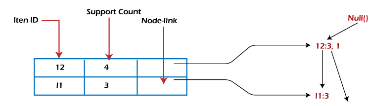
- Each node in the item-prefix subtree consists of three fields:
- Item-name: registers which item is represented by the node;
- Count: the number of transactions represented by the portion of the path reaching the node;
- Node-link: links to the next node in the FP-tree carrying the same item name or null if there is none.
- Each entry in the frequent-item-header table consists of two fields:
- Item-name: as the same to the node;
- Head of node-link: a pointer to the first node in the FP-tree carrying the item name.
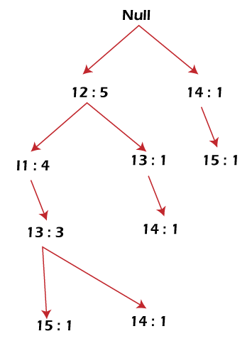
Additionally, the frequent-item-header table can have the count support for an item. The below diagram is an example of a best-case scenario that occurs when all transactions have the same itemset; the size of the FP-tree will be only a single branch of nodes.
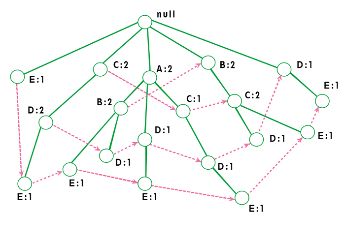
The worst-case scenario occurs when every transaction has a unique item set. So the space needed to store the tree is greater than the space used to store the original data set because the FP-tree requires additional space to store pointers between nodes and the counters for each item. The diagram below shows how a worst-case scenario FP-tree might appear. As you can see, the tree's complexity grows with each transaction's uniqueness.
Algorithm by Han
The original algorithm to construct the FP-Tree defined by Han is given below:
Algorithm 1: FP-tree construction
Input: A transaction database DB and a minimum support threshold?
Output: FP-tree, the frequent-pattern tree of DB.
Method: The FP-tree is constructed as follows.
- The first step is to scan the database to find the occurrences of the itemsets in the database. This step is the same as the first step of Apriori. The count of 1-itemsets in the database is called support count or frequency of 1-itemset.
- The second step is to construct the FP tree. For this, create the root of the tree. The root is represented by null.
- The next step is to scan the database again and examine the transactions. Examine the first transaction and find out the itemset in it. The itemset with the max count is taken at the top, and then the next itemset with the lower count. It means that the branch of the tree is constructed with transaction itemsets in descending order of count.
- The next transaction in the database is examined. The itemsets are ordered in descending order of count. If any itemset of this transaction is already present in another branch, then this transaction branch would share a common prefix to the root.
This means that the common itemset is linked to the new node of another itemset in this transaction.
- Also, the count of the itemset is incremented as it occurs in the transactions. The common node and new node count are increased by 1 as they are created and linked according to transactions.
- The next step is to mine the created FP Tree. For this, the lowest node is examined first, along with the links of the lowest nodes. The lowest node represents the frequency pattern length 1. From this, traverse the path in the FP Tree. This path or paths is called a conditional pattern base.
A conditional pattern base is a sub-database consisting of prefix paths in the FP tree occurring with the lowest node (suffix).
- Construct a Conditional FP Tree, formed by a count of itemsets in the path. The itemsets meeting the threshold support are considered in the Conditional FP Tree.
- Frequent Patterns are generated from the Conditional FP Tree.
Using this algorithm, the FP-tree is constructed in two database scans. The first scan collects and sorts the set of frequent items, and the second constructs the FP-Tree.
Example
Support threshold=50%, Confidence= 60%
Table 1:
| Transaction |
List of items |
| T1 |
I1,I2,I3 |
| T2 |
I2,I3,I4 |
| T3 |
I4,I5 |
| T4 |
I1,I2,I4 |
| T5 |
I1,I2,I3,I5 |
| T6 |
I1,I2,I3,I4 |
Solution: Support threshold=50% => 0.5*6= 3 => min_sup=3
Table 2: Count of each item
| Item |
Count |
| I1 |
4 |
| I2 |
5 |
| I3 |
4 |
| I4 |
4 |
| I5 |
2 |
Table 3: Sort the itemset in descending order.
| Item |
Count |
| I2 |
5 |
| I1 |
4 |
| I3 |
4 |
| I4 |
4 |
Build FP Tree
Let's build the FP tree in the following steps, such as:
- Considering the root node null.
- The first scan of Transaction T1: I1, I2, I3 contains three items {I1:1}, {I2:1}, {I3:1}, where I2 is linked as a child, I1 is linked to I2 and I3 is linked to I1.
- T2: I2, I3, and I4 contain I2, I3, and I4, where I2 is linked to root, I3 is linked to I2 and I4 is linked to I3. But this branch would share the I2 node as common as it is already used in T1.
- Increment the count of I2 by 1, and I3 is linked as a child to I2, and I4 is linked as a child to I3. The count is {I2:2}, {I3:1}, {I4:1}.
- T3: I4, I5. Similarly, a new branch with I5 is linked to I4 as a child is created.
- T4: I1, I2, I4. The sequence will be I2, I1, and I4. I2 is already linked to the root node. Hence it will be incremented by 1. Similarly I1 will be incremented by 1 as it is already linked with I2 in T1, thus {I2:3}, {I1:2}, {I4:1}.
- T5:I1, I2, I3, I5. The sequence will be I2, I1, I3, and I5. Thus {I2:4}, {I1:3}, {I3:2}, {I5:1}.
- T6: I1, I2, I3, I4. The sequence will be I2, I1, I3, and I4. Thus {I2:5}, {I1:4}, {I3:3}, {I4 1}.
Mining of FP-tree is summarized below:
- The lowest node item, I5, is not considered as it does not have a min support count. Hence it is deleted.
- The next lower node is I4. I4 occurs in 2 branches , {I2,I1,I3:,I41},{I2,I3,I4:1}. Therefore considering I4 as suffix the prefix paths will be {I2, I1, I3:1}, {I2, I3: 1} this forms the conditional pattern base.
- The conditional pattern base is considered a transaction database, and an FP tree is constructed. This will contain {I2:2, I3:2}, I1 is not considered as it does not meet the min support count.
- This path will generate all combinations of frequent patterns : {I2,I4:2},{I3,I4:2},{I2,I3,I4:2}
- For I3, the prefix path would be: {I2,I1:3},{I2:1}, this will generate a 2 node FP-tree : {I2:4, I1:3} and frequent patterns are generated: {I2,I3:4}, {I1:I3:3}, {I2,I1,I3:3}.
- For I1, the prefix path would be: {I2:4} this will generate a single node FP-tree: {I2:4} and frequent patterns are generated: {I2, I1:4}.
| Item |
Conditional Pattern Base |
Conditional FP-tree |
Frequent Patterns Generated |
| I4 |
{I2,I1,I3:1},{I2,I3:1} |
{I2:2, I3:2} |
{I2,I4:2},{I3,I4:2},{I2,I3,I4:2} |
| I3 |
{I2,I1:3},{I2:1} |
{I2:4, I1:3} |
{I2,I3:4}, {I1:I3:3}, {I2,I1,I3:3} |
| I1 |
{I2:4} |
{I2:4} |
{I2,I1:4} |
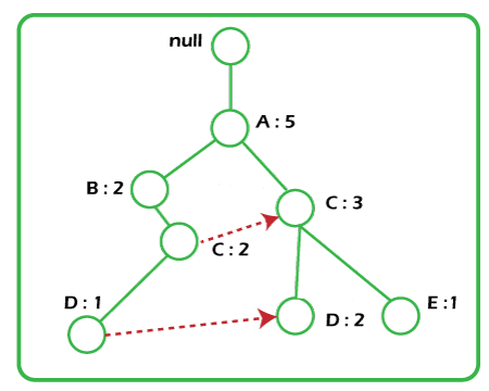
The diagram given below depicts the conditional FP tree associated with the conditional node I3.
FP-Growth Algorithm
After constructing the FP-Tree, it's possible to mine it to find the complete set of frequent patterns. Han presents a group of lemmas and properties to do this job and then describes the following FP-Growth Algorithm.
Algorithm 2: FP-Growth
Input: A database DB, represented by FP-tree constructed according to Algorithm 1, and a minimum support threshold?
Output: The complete set of frequent patterns.
Method: Call FP-growth (FP-tree, null).
When the FP-tree contains a single prefix path, the complete set of frequent patterns can be generated in three parts:
- The single prefix-path P,
- The multipath Q,
- And their combinations (lines 01 to 03 and 14).
The resulting patterns for a single prefix path are the enumerations of its subpaths with minimum support. After that, the multipath Q is defined, and the resulting patterns are processed. Finally, the combined results are returned as the frequent patterns found.
Advantages of FP Growth Algorithm
Here are the following advantages of the FP growth algorithm, such as:
- This algorithm needs to scan the database twice when compared to Apriori, which scans the transactions for each iteration.
- The pairing of items is not done in this algorithm, making it faster.
- The database is stored in a compact version in memory.
- It is efficient and scalable for mining both long and short frequent patterns.
Disadvantages of FP-Growth Algorithm
This algorithm also has some disadvantages, such as:
- FP Tree is more cumbersome and difficult to build than Apriori.
- It may be expensive.
- The algorithm may not fit in the shared memory when the database is large.
Difference between Apriori and FP Growth Algorithm
Apriori and FP-Growth algorithms are the most basic FIM algorithms. There are some basic differences between these algorithms, such as:
| Apriori |
FP Growth |
| Apriori generates frequent patterns by making the itemsets using pairings such as single item set, double itemset, and triple itemset. |
FP Growth generates an FP-Tree for making frequent patterns. |
| Apriori uses candidate generation where frequent subsets are extended one item at a time. |
FP-growth generates a conditional FP-Tree for every item in the data. |
| Since apriori scans the database in each step, it becomes time-consuming for data where the number of items is larger. |
FP-tree requires only one database scan in its beginning steps, so it consumes less time. |
| A converted version of the database is saved in the memory |
A set of conditional FP-tree for every item is saved in the memory |
| It uses a breadth-first search |
It uses a depth-first search. |
|

 For Videos Join Our Youtube Channel: Join Now


