| |

MATLAB InterpolationInterpolation is the process of describing a function which "connects the dots" between specified (data) points. The most common interpolation technique is Linear Interpolation. A more exotic interpolation scheme is to link the data points using third degree or cubic polynomials. In MATLAB, we can interpolate our data using splines or Hermite interpolants on a fly. MATLAB provides the following functions to help interpolation: Let us understand these functions of MATLAB one by one: interp1One-dimensional data interpolation. Given yi at xi, finds yj at xj from yj=f(xj ). Here f is a continuous function that is seen from interpolation. It is called one-dimensional interpolation because y depends on a single variable x. Syntax ynew=interp1(x,y,xnew,method) where the method is an optional argument discussed after the description of interp2 and interp3. interp2Two-dimensional data interpolation. Given zi at (xi, yi), finds zj at desired (xj,yj )from z=f(x,y).The function f is found from interpolation. It is called two-dimensional interpolation because z depends on two variables, x, and y. Syntax znew=interp2(x,y,z,xnew,ynew,method). interp3Three-dimensional analogue of interp1. Given vi at (xi, yi,zi), finds vj at desired(xj,yj,zj). Syntax vnew=interp3(x,y,z,xnew,ynew,znew,method). Also, there is an n-dimensional analog, interpn, if you ever need it. In each function, we have the option of specifying a method of interpolation. The choice for the technique is nearest, linear, cubic, or spline. The choice of the method dictates the smoothness of the interpolated data. The default method is linear. To specify cubic interpolation instead of linear, for example, in interp1, use the syntax: ynew=interp1(x,y,xnew,' cubic' ). splineOne-dimensional interpolation that uses cubic splines to find yj at desired xj,given yi at xi. Cubic splines fit separate cubic polynomials between successive data points by matching the slopes as well as the curvature of each segment at the given data points. Syntax ynew=spline(x,y,xnew,method). interpfitFast Fourier Transform (FFT)-based 1-D data interpolation. This is similar to interp1 except that the data is interpolated first by taking the Fourier Transform of the given data and then calculating the inverse transform using more data points. The interpolation is especially useful for periodic functions (i.e., if values of y are periodic). Syntax y = interpft(X,n) ExampleThere are two simple steps contained in interpolation: providing a list (a vector) of points at which you wish to get interpolated data and executing the appropriate function (e.g., interp1) with the desired choice for the method of interpolation. We illustrate these steps through an example on the x and y data given in the following table:
Step1: Generate a vector xi containing desired points for interpolation. % take equally spaced fifty points. Step2: Generate data yi at xi. % generate yi at xi with cubic interpolation. Here 'cubic' is the choice for the interpolation scheme. The other schemes we could use are nearest, linear, and spline. The data generated by each scheme is shown in fig, along with the original input. 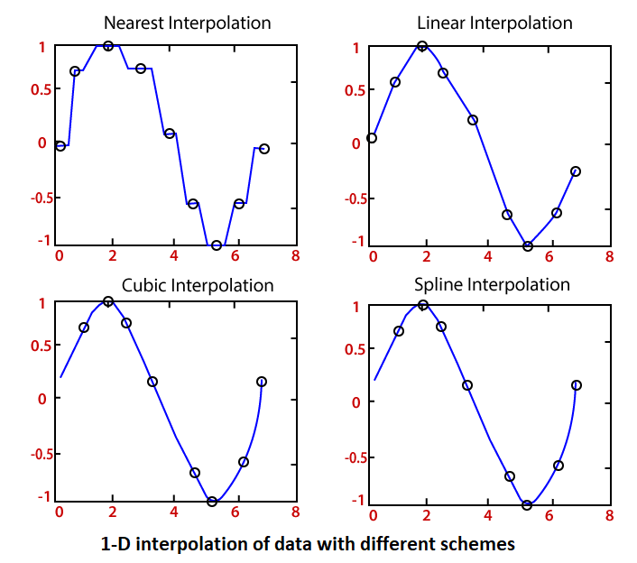
Next TopicNumerical Integration
|
 For Videos Join Our Youtube Channel: Join Now
Feedback
- Send your Feedback to [email protected]
Help Others, Please Share


