MATLAB Simpson's Rule

The trapezoidal and Simpson's rules are special cases of the Newton-Cote rules which use higher degree functions for numerical integration.

Let the parabola represent the curve of the figure.

y=αx²+βx+γ…………..equation 1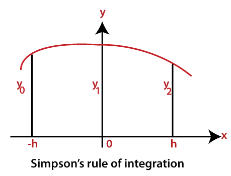

The area under this method for the interval -h≤x≤h is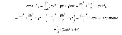

The curve passes through the three points(-h,y₀ ),(0,y₁ ),and (h,y₂ ). Then, by an equation, we have: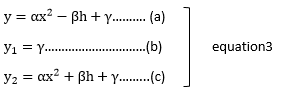

We can now evaluate the coefficients α,β,γ and express equation2 in terms of h, y₀, y₁and y₂.

By substitution of (b) of equation3 into (a) and (c) and rearranging we obtain

αx²-βh=y₀-y₁…..equation4

αx²+βh=y₂-y₁…..equation5

Adding of equation4 with equation 5 yields

2αh²=y₀-2y₁+y₂…...equation6

and by substitution into equation2, we obtain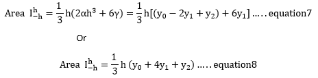

Now, we can apply equation8 to successive segments of any curve y=f(x) in the interval a≤x≤b as shown on the curve of the figure.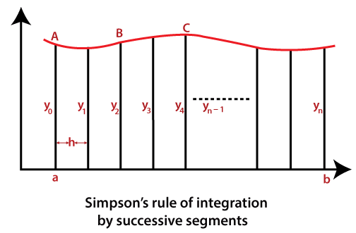

We observe that a parabola can approximate each segment of width 2h of the curve through its ends and its midpoint. Thus, the area under segment AB is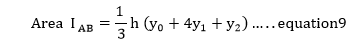

Likewise, the area under segment BC is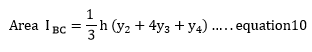

and so on. When the areas under each segment are added, we obtain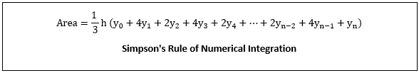

Since each segment has width 2h, to apply Simpson's rule of numerical integration, the number n of subdivisions must be even. This restriction does not apply to the trapezoidal rule of numerical integration.

The value of for equation11 is found from