Kalman Filter Matlab

Introduction to Kalman Filter Matlab

One method for estimating a system's state from a set of noisy measurements is the Kalman filter algorithm. When the system is dealing with erratic, noisy, or partial data, it is especially helpful.

The filter's method of operation involves iteratively estimating the system's state at each time step using a forecast of the state and its corresponding uncertainty, then updating the estimate with fresh data. Numerous industries, including navigation, signal processing, and control systems, make extensive use of it.

Understanding and Implementing the Kalman Filter in MATLAB

A strong and adaptable instrument, the Kalman filter is employed in signal processing, navigation, control systems, and other domains. It is especially useful in situations when you have to use noisy measurements to estimate the status of a dynamic system. This article covers the basic principles of the Kalman filter and offers a detailed tutorial for using it in MATLAB.

The Kalman filter is a state-space estimating technique that is recursive and was created by Rudolf E. Kalman in the 1960s. It is frequently used, particularly when working with noisy or imperfect data, to track and estimate the state of dynamic systems. The Kalman filter's main objective is to estimate a system's current state by fusing fresh observations with the system's prior state estimate.

The Kalman filter operates under two essential assumptions:

The system is linear, meaning its dynamics can be modeled using linear equations.

The noise in the system, both in the process and measurement, follows Gaussian distributions. In practice, while the Kalman filter works best with linear systems, it can be extended to handle nonlinear systems through variations like the Extended Kalman Filter (EKF) and Unscented Kalman Filter (UKF).

The Kalman filter can be broken down into two fundamental steps:

"Prediction and Correction"

These steps are performed iteratively to estimate the current state of the system.

Prediction:

• Based on the system dynamics and the estimated prior state, predict the upcoming state.
• Estimate the estimation error's covariance.
• Because it forecasts the state and its uncertainty into the future based on the dynamics of the system, the prediction step is crucial.

Correction:

• Get a fresh measurement from the apparatus.
• To find the Kalman Gain, compare the measurement and the expected state.
• Apply Kalman Gain to the state estimation update.
• Reload the estimation error's covariance.
• The purpose of the corrective step is to improve the state estimate by using fresh measurements.

Kalman Filter Equations

To implement the Kalman filter in MATLAB, it's crucial to understand the underlying equations:

State Prediction:

State Prediction Equation:

xk =A⋅xk-1 +B-uk +wk

Here:

xk: Predicted state at time k

A: State transition matrix

xk-1: Previous state estimate at time k-1

B: Control input matrix

uk: Control input at time k

wk: Process noise at time k

Covariance Prediction Equation:

The state vector in this case is represented by x, the state transition matrix by A, the control input matrix by B (you are the control input), the process noise covariance matrix by Q, and the state estimate covariance matrix by P.

Pk =A⋅Pk-1 ⋅AT+Q

Here:

Pk: The state's anticipated covariance at time k

A: matrix of state transitions

Pk-1: The state's prior covariance at time k-1.

Q: Noise covariance matrix processing

By considering the dynamics of the system and the process noise, this equation forecasts the covariance of the state estimate at the subsequent time step.

State Correction:

Kalman Gain Equation:

The weight assigned to the new measurement in adjusting the state estimate is determined by the Kalman Gain. It plays a critical role in distributing the impact of the new measurement and the prediction.

Kk =Pk ⋅HT⋅(H⋅Pk ⋅HT+R)-1

KK: Kalman Gain at time k

Pk: The state's anticipated covariance at time k

H: Matrix of measurements

R: Matrix of measurement noise covariance

The Kalman Gain can be computed by scaling the projected covariance with the transpose of the measurement matrix and the inverse of the innovation covariance (the term in parentheses). It represents how sensitive the system is to the new measurement.

State Correction Equation:

xk =xk +Kk ⋅(zk -H⋅xk )

Xk: Corrected state estimate at time k

Kk : Kalman Gain at time k

zk: Actual measurement at time k

H: Measurement matrix

Covariance Correction Equation:

In these equations, K is the Kalman Gain, H is the measurement matrix, R is the measurement noise covariance matrix, and z is the measurement vector.

Pk =(I-Kk ⋅H)⋅Pk

Pk: Corrected covariance of the state at time k

Kk : Kalman Gain at time k

H: Measurement matrix

I: Identity matrix

Kalman Gain: The computation of the Kalman Gain takes into account the uncertainty in both the measurement (H⋅Pk ⋅HT+R) and the anticipated state (Pk). The smaller the Kalman Gain, indicating less reliance on the new measurement, the greater the uncertainty in the forecast in relation to the measurement's uncertainty.

State Correction: The difference between the actual measurement (zk) and the expected measurement (H⋅xk) is the innovation, and it is used to change the predicted state (xk) based on the innovation and the Kalman Gain.

Covariance Correction: To account for the accuracy of the corrected state estimate, the predicted covariance (Pk) is modified using the Kalman Gain. The proper scaling of the covariance is guaranteed by the expression I-Kk ⋅H.

Example:

Output: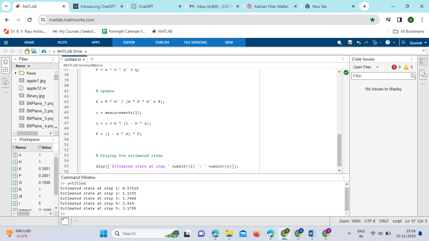

• Even in the face of noise and uncertainty, the Kalman filter proves to be a potent instrument for determining the state of dynamic systems.
• Tracking moving objects and estimating system states in control systems are only two of the many uses for the Kalman filter that may be achieved by comprehending the prediction and correction processes and the corresponding equations. You may fully utilize the possibilities of this adaptable estimating technique with practice and fine-tuning.

Advantages and Disadvantages

A Recursive technique called the Kalman filter uses a sequence of noisy observations to estimate the state of a linear dynamic system. It is extensively utilized in many different domains, such as navigation, control systems, and signal processing.

Advantages:

Optimal Estimation: In the presence of Gaussian noise, the Kalman filter yields the best estimate of the state of a linear dynamic system. It reduces the estimate's mean squared error.

Adaptability: The Kalman filter can handle parameters that change over time and is flexible enough to work with a variety of systems. On the basis of fresh measurements and system dynamics, it can modify its estimates.

Efficiency: The Kalman filter is computationally efficient, making it suitable for real-time applications. MATLAB provides built-in functions for Kalman filtering, making it easy to implement and use.

Handling of Sensor Noise: The Kalman filter is designed to handle measurements with noise. It effectively combines information from the system dynamics (predictive model) and noisy measurements to provide a more accurate state estimate.

Recursive Nature: The filter is recursive, meaning that it updates its estimate based on the latest measurements and predictions. This makes it well-suited for online or real-time applications.

State Estimation for Unobservable Variables: The Kalman filter can estimate the state of variables that are not directly measurable. It can infer the values of these unobservable variables based on the available measurements.

Disadvantages:

Linearity Assumption: Linear dynamic systems are the target application for the Kalman filter. The Extended Kalman Filter (EKF) or the Unscented Kalman Filter (UKF) may be necessary if the system is extremely nonlinear in order for the filter to function properly.

Sensitivity to Model Mismatch: The accuracy of the system model affects how well the Kalman filter performs. Should there be a notable discrepancy between the model and the real system, the filter might yield less-than-ideal outcomes.

Noise Assumption: The Kalman filter operates under the assumption that the noise present in the system is Gaussian. In actuality, the efficiency of the filter could be impacted if the noise differs considerably from the Gaussian distribution.

Complexity for Non-Experts: For people who need to learn more about the underlying mathematical ideas, implementing and fine-tuning a Kalman filter can be difficult. Users might require a solid grasp of measurement models and system dynamics.

Memory Requirements: In applications with limited memory, the Kalman filter may require significant storage for maintaining covariance matrices and other variables.

Initialization Sensitivity: The initial conditions and covariance values can significantly impact the filter's performance. Choosing appropriate initial values requires some understanding of the system and may involve some trial and error.