Matlab Autocorrelation

Introduction

Autocorrelation is a fundamental concept in signal processing, revealing inherent patterns within a signal by measuring its similarity to a time-shifted version of itself. In MATLAB, autocorrelation plays a pivotal role in various applications, offering insights into signal characteristics and aiding in diverse fields.

Understanding Autocorrelation

Autocorrelation, in simple terms, involves comparing a signal with its delayed version. This process is instrumental in identifying repeating patterns and extracting valuable information from time-series data.

• Autocorrelation, a fundamental concept in signal processing, unveils intricate details within a signal by examining its similarity to a time-shifted version of itself.

Autocorrelation Fundamentals

At its core, autocorrelation is a measure of similarity between a signal, and a version of itself shifted in time.

Mathematically, the autocorrelation function R(τ) for a continuous signal x(t) is defined as:

For discrete signals, the autocorrelation function is given

Here, τ represents the time shift, and k is the discrete lag.

Basic Autocorrelation Implementation

Basic autocorrelation implementation in MATLAB involves computing the autocorrelation function of a given signal and visualizing the result.

• Autocorrelation is a fundamental operation in signal processing that measures the similarity between a signal and a time-shifted version of itself.

To begin with, let's consider a simple example: We generate a random signal and compute its autocorrelation using the xcorr function in MATLAB.

Example:

Output: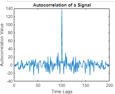

Explanation:

We create a random signal of length 100 using randn. The xcorr function computes the signal's autocorrelation. The resulting autocorrelation values are plotted against time lags.

Identifying Autocorrelation Peaks

In MATLAB, the findpeaks function is commonly used to locate peaks in the autocorrelation function.

• By analyzing the autocorrelation results, researchers and practitioners can identify significant features in the signal, such as fundamental frequencies or dominant harmonics.
• These peaks provide valuable insights into the signal's underlying structure and characteristics, facilitating further analysis and interpretation.

The findpeaks function in MATLAB can assist in this task.

Example:

Output: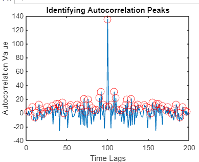

Moreover, visualizing autocorrelation peaks allows for a clear representation of the signal's periodic components.

• MATLAB's plotting capabilities enable users to overlay peaks on the autocorrelation graph, providing a visual reference for the identified features.
• By examining the distribution and magnitude of peaks, analysts can gain a deeper understanding of the signal's behavior and make informed decisions in signal processing tasks.

Explanation:

The findpeaks function is used to locate peaks in the autocorrelation function. Peaks are then plotted on the autocorrelation graph, providing a visual representation of significant features.

Customizing Autocorrelation Plots

MATLAB allows users to customize autocorrelation plots for enhanced clarity and insight.

Customization Parameters:

Line Width:

Adjusting the line width helps emphasize the autocorrelation curve, making it more prominent and easier to distinguish from other elements in the plot.

Color:

Choosing an appropriate color scheme enhances the visual appeal and clarity of the plot. MATLAB allows specifying colors using RGB values or predefined color names.

Grid Display:

Enabling grid lines on the plot provides additional reference points, aiding in the accurate interpretation of autocorrelation values at different time lags.

Here's an example of how to customize the plot:

Output:

Explanation:

The LineWidth and Color options adjust the appearance of the autocorrelation plot. Grid on adds a grid to the plot for better readability.

Advanced Autocorrelation Techniques

For more advanced applications, MATLAB provides additional techniques, such as using window functions or Fourier Transform-based methods.

Window Functions for Improved Accuracy

• Applying window functions before computing autocorrelation can mitigate edge effects and improve accuracy, especially for finite-duration signals.
• Widely used windows include Hamming, Hann, and Blackman-Harris.
• These windows taper the signal's edges, reducing spectral leakage and providing a more reliable autocorrelation result.

MATLAB provides various window functions, and here we'll demonstrate the use of the Hamming window:

Output: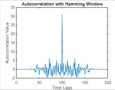

The signal is multiplied element-wise with the Hamming window using. The core function is then applied to the windowed signal, providing a more accurate autocorrelation result.

Multivariate Autocorrelation:

Extending autocorrelation to multivariate signals allows for analyzing relationships between multiple time-series variables. Multivariate autocorrelation techniques, such as cross-covariance and cross-correlation matrices, enable the examination of interdependencies and lagged relationships between different variables, offering insights into complex systems' dynamics.

Example:

Output: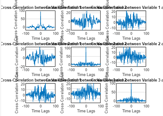

Explanation:

• We generate example multivariate time-series data (data) with 100 samples and 3 variables.
• We compute the cross-correlation matrix (cross_corr_matrix) by iterating over all pairs of variables and computing their cross-correlation using the xcorr function.
• Finally, we plot the cross-correlation matrices for each pair of variables, displaying the cross-correlation values across different time lags.

Frequency-Domain Autocorrelation:

Transforming signals into the frequency domain via Fourier Transform-based methods provides an alternative approach to autocorrelation analysis.

• Autocorrelation in the frequency domain involves computing the power spectral density (PSD) and extracting autocorrelation information indirectly from the frequency components.
• This technique is particularly useful for analyzing signals with distinct frequency components or periodic behavior.

Example:

Output: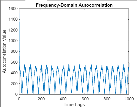

Explanation:

• We generate an example signal consisting of a sinusoidal component with added noise.
• The Fourier Transform of the signal is computed using fft.
• The squared magnitude of the Fourier Transform yields the Power Spectral Density (PSD).
• We then take the Inverse Fourier Transform of the PSD (ifft) to obtain the autocorrelation function in the time domain.
• Finally, we plot the autocorrelation function to visualize the results.

Time-Frequency Autocorrelation:

Incorporating time-frequency analysis methods, such as wavelet transforms or spectrograms, allows for examining autocorrelation dynamics across both time and frequency domains.

• Time-frequency autocorrelation techniques provide a more comprehensive understanding of signal characteristics, capturing transient features and frequency changes over time, which may be missed in traditional autocorrelation analysis.

Example:

Output: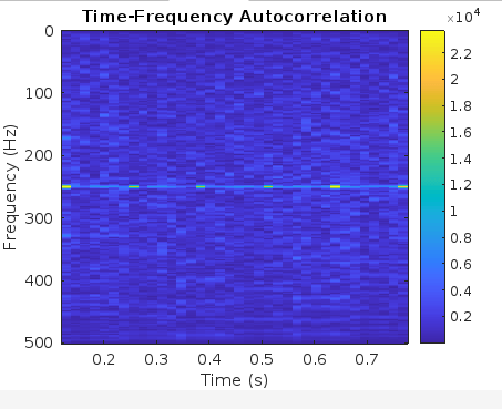

Explanation:

• We generate an example signal consisting of a sinusoidal component with added noise.
• We define parameters for the spectrogram, including window size and overlap.
• The spectrogram of the signal is computed using the spectrogram function.
• We compute the autocorrelation of the spectrogram using the score function.

Fourier Transform-based approach:

The Fourier Transform provides a powerful tool for analyzing signals in the frequency domain. In the context of autocorrelation, we can leverage the Fourier Transform to compute the autocorrelation function indirectly.

Steps for Fourier Transform-based Autocorrelation:

Compute the Fourier Transform:

Begin by computing the Fourier Transform of the signal of interest. The Fourier Transform decomposes the signal into its frequency components, revealing the signal's spectral content.

Compute Power Spectral Density (PSD):

Square the magnitude of the Fourier Transform to obtain the Power Spectral Density (PSD). The PSD represents the distribution of signal power across different frequencies.

Inverse Fourier Transform (IFT):

Take the Inverse Fourier Transform of the squared magnitude to obtain the autocorrelation function in the time domain. This step effectively converts the frequency domain representation back to the time domain.

Example:

Output: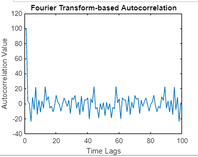

Explanation:

The Fourier Transform-based autocorrelation involves taking the inverse Fourier Transform of the squared magnitude of the signal's Fourier Transform. This technique provides an alternative perspective on autocorrelation, useful in certain scenarios.