Matlab Gradient

Introduction:

MATLAB, a versatile programming language and computational environment, stands at the forefront of scientific computing, engineering, and data analysis. With its rich set of built-in functions and toolboxes, MATLAB facilitates the exploration and manipulation of mathematical models, making it an indispensable tool for researchers, engineers, and data scientists.

Among the myriad functionalities MATLAB offers, the concept of gradients plays a pivotal role in understanding the behavior of functions and datasets.

Understanding Gradients:

A gradient is a vector that points in the direction of the steepest increase of a scalar field. In simpler terms, it represents the slope of a function at a particular point. The Gradient is often denoted by the symbol ∇ (nabla) and is mathematically expressed as follows for a function f(x, y):

Here, ∂x∂f and ∂y∂f are the partial derivatives of the function f with respect to its independent variables x and y, respectively. The Gradient provides valuable information about the direction and magnitude of the fastest change in the function.

Applications of Gradients:

Gradients find applications in various fields, and their importance extends to different domains. Some notable applications include:

Optimization:

Gradients are essential in optimization problems where the goal is to find the minimum or maximum of a function. Algorithms such as gradient descent utilize the Gradient to iteratively update the parameters of a model to reach the optimal solution.

Machine Learning:

In machine learning, gradients are used in training algorithms to update model parameters. The Gradient of the loss function with respect to the model parameters guides the learning process, helping the algorithm converge to an optimal solution.

Image Processing:

Gradients are employed in edge detection algorithms to identify boundaries and transitions between different regions in an image. The magnitude and direction of the Gradient at each pixel provide valuable information for image analysis.

Physics and Engineering:

Gradients are extensively used in physics and engineering simulations to model the behavior of physical systems. They help analyze the flow of heat, fluid dynamics, and other dynamic processes.

MATLAB Gradient Functions:

MATLAB provides several built-in functions to compute gradients efficiently. Some of the key functions include:

Gradient:

The gradient function in MATLAB computes the numerical Gradient of a vector or scalar function. It is particularly useful when dealing with discrete data. For example:

This code calculates the Gradient of the sine function with respect to x.

gradient2:

The gradient2 function extends the concept of the Gradient to two-dimensional grids. It computes the gradients along the rows and columns of a matrix.

For example:

Here, Gx and Gy represent the gradients of the function Z with respect to X and Y, respectively.

griddedInterpolant:

The griddedInterpolant function is useful for interpolating values on a grid. By calculating gradients at interpolated points, this function aids in creating smooth surfaces from scattered data.

Here, Xq and Yq represent the interpolated grid, and Zq is the corresponding interpolated surface.

Quiver:

The quiver function is useful for visualizing vector fields, such as gradients. It can be employed to visualize the direction and magnitude of gradients at specific points.

This code generates a quiver plot representing the gradients of the function Z.

Implementation:

Calculating Gradient with Gradient:

Output: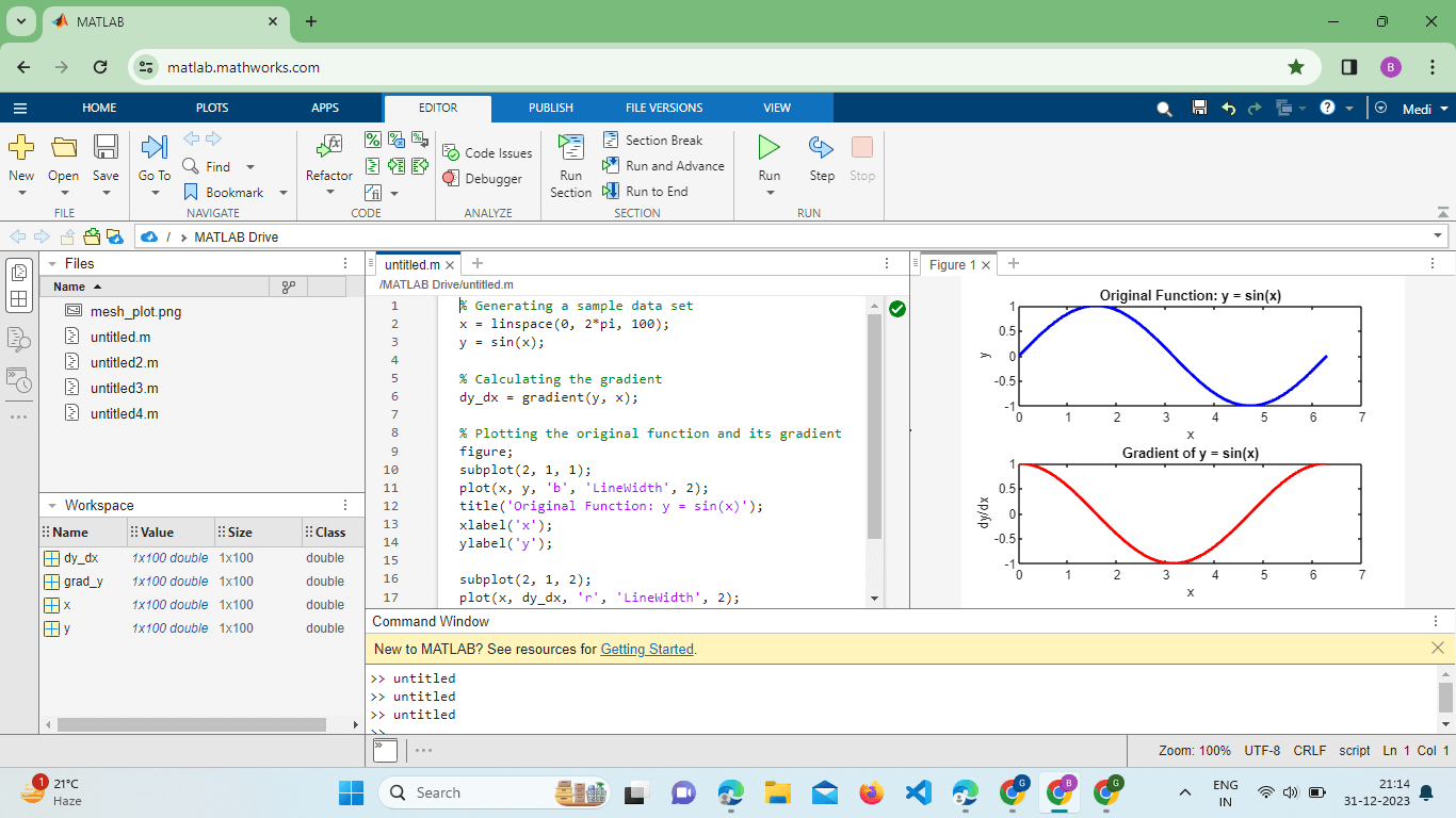

Explanation:

We create a figure with two subplots arranged vertically. In the first subplot (top), we plot the original sine function (y = sin(x)) using a blue line ('b') with a line width of 2. The title and axis labels are added for clarity.

• In the second subplot (bottom), we plot the calculated Gradient (dy_dx) using a red line ('r') with a line width of 2. Again, a title and axis labels are included.
• The resulting visualization allows you to compare the original sine function with its Gradient.
• The top subplot shows the sine curve, while the bottom subplot illustrates how the Gradient varies across the range of x.
• The gradient plot represents the rate of change of the sine function at each point. As x increases, the gradient plot shows where the sine function is steepest (peaks and troughs).

Program2:

Visualizing Vector Fields with Quiver:

Output: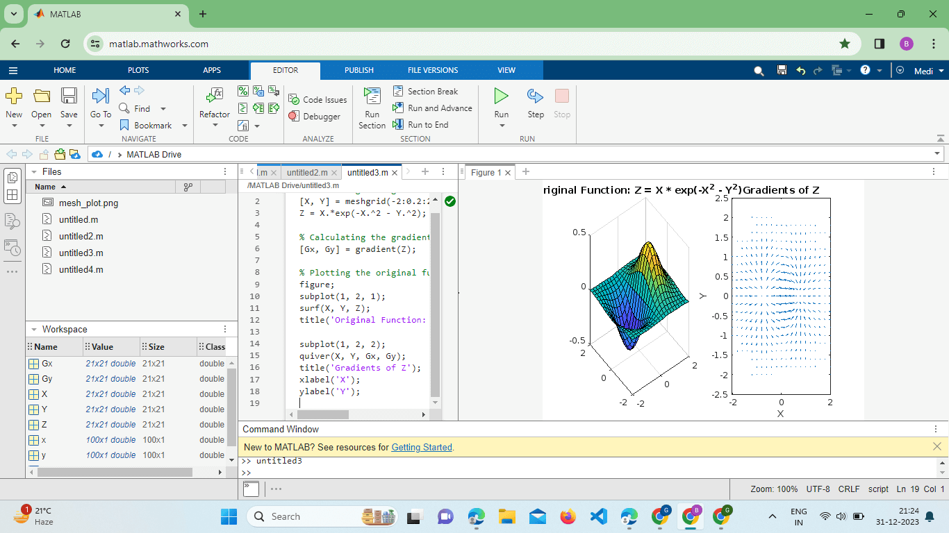

MATLAB's gradient functions, such as Gradient, gradient2, griddedInterpolant, and quiver, provide powerful tools for efficiently calculating and visualizing gradients.

• Whether you're working on optimization problems, machine learning applications, image processing, or simulations in physics and engineering, understanding and leveraging
• MATLAB's gradient functions can significantly enhance your ability to analyze and interpret data.
• As you delve deeper into MATLAB's capabilities, experimenting with these gradient functions will empower you to tackle a wide range of real-world problems, making MATLAB an invaluable tool in your computational toolkit.