Matlab ksdensity

Introduction

Kernel density estimation (KDE) is a non-parametric way to estimate the probability density function of a random variable. It is a powerful statistical tool used in various fields, such as data analysis, machine learning, and signal processing.

• The term "ksdensity" often refers to the kernel density estimation function provided by MATLAB, which allows users to compute and visualize kernel density estimates.

Basic Concept:

Kernel density estimation is a method used to estimate the probability density function (PDF) of a random variable. It involves placing a kernel (a smooth, usually bell-shaped, function) on each data point and summing up these kernels to obtain a smooth estimate of the underlying distribution.

Syntax:

The syntax of the ksdensity function in MATLAB is as follows:

Where data is the input data vector, f is the estimated density values corresponding to evaluation points x.

What is Kernel Function?

A kernel function, in the context of kernel density estimation (KDE) and other kernel-based methods, is a mathematical function that determines the shape and weight of the contribution of each data point to the estimation of the underlying probability density function (PDF).

Here's a breakdown of its key characteristics:

Shape: Kernel functions are typically symmetric, non-negative functions centered at zero. They define the shape of the kernel used to smooth the data. Common kernel shapes include bell-shaped (e.g., Gaussian), flat-top (e.g., Epanechnikov), and triangular.

Weight: The kernel function assigns weights to data points based on their distance from the point of interest (usually the point at which the density estimate is being evaluated). Points closer to the center have higher weights, indicating a stronger influence on the density estimate.

Bandwidth: The bandwidth parameter determines the width of the kernel, controlling the level of smoothing applied to the density estimate. A larger bandwidth results in a smoother estimate, while a smaller bandwidth captures more detail in the data but may introduce more noise.

Types of Kernel Functions:

There are several types of kernel functions commonly used in kernel density estimation, each with its properties and characteristics:

1. Gaussian Kernel: The Gaussian (normal) kernel is the most widely used and has a bell-shaped curve.
2. Epanechnikov Kernel: This kernel has a flat-top shape and is often used for its efficient properties.
3. Triangular Kernel: The triangular kernel has a triangular shape and is another commonly used option.

Choice of Kernel:

The choice of kernel depends on the specific characteristics of the data and the desired properties of the density estimate. Different kernels may perform better or worse depending on the dataset's distribution and the underlying assumptions.

Kernel Normalization:

In some cases, kernel functions are normalized to integrate into one, ensuring that the estimated density is a proper probability density function. This normalization ensures that the area under the estimated density curve equals one, making it interpretable as a probability.

Customizing KDE with ksdensity

Choosing Kernel and Bandwidth

Users can specify the type of kernel function ('Kernel' parameter) and the bandwidth ('Bandwidth' parameter) to customize the KDE according to their data and analysis requirements. Common kernel options include Gaussian, Epanechnikov, and triangular kernels.

Specifying Evaluation Points

Users can also specify the set of evaluation points where the density estimate should be computed. This allows for fine-tuning the resolution and range of the estimated density.

Example:

Output: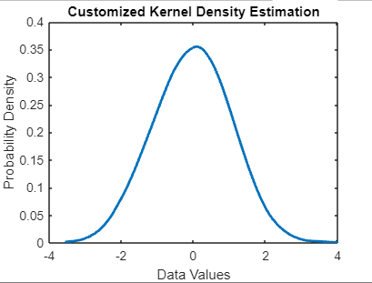

In this program:

• We generate synthetic data using randn.
• We specify the type of kernel function (kernel_type) as 'epanechnikov' and the bandwidth (bandwidth_value) as 0.5.
• We specify the set of evaluation points (evaluation_points) using linspace to generate points from -3 to 3 with a total of 100 points.
• We use ksdensity with the specified kernel, bandwidth, and evaluation points to perform kernel density estimation.

Visualizing KDE Results

Once the density estimate is obtained using ksdensity, users can visualize the results using MATLAB's plotting functions. Common visualization methods include line plots, histograms, and surface plots, depending on the dimensionality of the data and the desired level of detail.

Example:

Output:

In this program:

• We generate synthetic data using randn.
• We perform kernel density estimation using ksdensity.
• The ksdensity function returns the estimated density (estimated_density) and the corresponding evaluation points (x_values).
• We then plot the estimated density using a plot, with the evaluation points on the x-axis and the estimated density values on the y-axis.

Applications of KDE with ksdensity

Data Exploration

KDE with ksdensity is widely used for exploring the distribution of a dataset, providing insights into the underlying structure and patterns present in the data.

Density Comparison

It enables the comparison of densities between different datasets, facilitating the identification of similarities, differences, and patterns across datasets.

Anomaly Detection

KDE can be used for anomaly detection by identifying regions with low probability density. Density helps detect outliers or anomalies in the data, which may indicate unusual or unexpected behavior.

Non-Parametric Regression

Beyond density estimation, KDE with ksdensity can be utilized for non-parametric regression to estimate the relationship between variables. It offers a flexible approach to modeling complex relationships without assuming a specific functional form.

Example:

Output: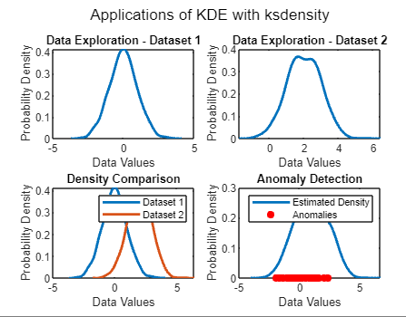

Explanation:

Data Exploration:

• Two synthetic datasets, data1 and data2, are generated using random numbers.
• Kernel density estimation is performed separately for each dataset.
• The estimated densities for both datasets are plotted in separate subplots, providing insights into each dataset's distribution.

Density Comparison:

• The estimated densities for both datasets (data1 and data2) are plotted on the same graph for comparison.
• This allows visual comparison of the distributions of the two datasets to identify similarities and differences.

Anomaly Detection:

• The two datasets (data1 and data2) are concatenated into a single dataset (combined_data).
• Kernel density estimation is performed for the combined dataset.
• Anomalies are identified as data points with estimated densities below a specified threshold (threshold).
• Anomalies are visualized on the plot as red filled circles, highlighting potential outliers or unusual data points.

Non-Parametric Regression:

• This application is mentioned but needs to be implemented in the script.
• Non-parametric regression using KDE goes beyond density estimation and can be used to estimate the relationship between variables.
• However, implementing non-parametric regression requires additional code beyond the capabilities of density.

Best Practices and Considerations

Bandwidth Selection

Choosing an appropriate bandwidth is crucial for obtaining an accurate density estimate. Users should experiment with different bandwidth values and consider cross-validation techniques to determine the optimal bandwidth for their dataset.

Kernel Selection

The choice of kernel function also impacts the quality of the density estimate. Users should consider the characteristics of their data and the desired properties of the estimate when selecting the kernel function.

Computational Efficiency

For large datasets, optimizing the computational efficiency of KDE algorithms becomes important. MATLAB offers efficient implementations of KDE algorithms, but users should be mindful of computational resources and algorithm complexity.