Linear fit MATLAB

Introduction:

The robust numerical computing environment MATLAB offers an extensive toolkit for data analysis and visualization. One of MATLAB's numerous features is its strong support for linear fitting, which lets users model the relationships between variables and do regression analysis. Understanding the foundations of linear fitting in MATLAB is crucial for any level of data analyst to enable them to make well-informed judgments based on insights from their data.

We will examine the fundamentals of linear fitting in MATLAB in this introduction, going over important ideas, methods of application, and real-world uses for linear regression. After finishing this primer, you'll have a firm grasp of how to use MATLAB's extensive function and capability set to apply linear fitting to your data analysis assignments.

Matlab's Linear Fit function works with syntax

Several functions in MATLAB can be used to perform linear fitting; polyfill is the most often used tool. Using the least squares method, the poly fit function fits the data with a polynomial. In particular, poly fit fits a first-degree polynomial, or a straight line, to the provided data points for linear fitting.

Syntax:

Where

The vector of data points for the independent variable is called x.

Y=The dependent variable data points' vector is denoted by y.

N=The degree of the polynomial fit, denoted by n (which is set to 1 for a linear fit).

The function yields the polynomial fit coefficients, which are useful in determining the linear equation's slope and y-intercept.

In addition, the polyval function can be used to create a fitted line using the coefficients that you acquired from polyfit or to evaluate the polynomial at particular places.

The following is the standard syntax for using polyval:

Where:

P=The vector of coefficients that Polyfit produced is denoted by p.

The vector of data points for the independent variable is called x.

You can effectively do regression analysis and linear fitting by learning and using these MATLAB algorithms.

An illustration of how to use these functions is provided below:

Example:

Output: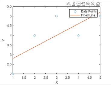

Linear Fit in MATLAB Understanding

In statistics and data analysis, linear fitting, commonly referred to as linear regression, is a fundamental approach.

• The link between a dependent variable and one or more independent variables is modeled using it. The simple technique of linear fitting in MATLAB enables users to analyze data, forecast outcomes, and derive insights from the data.
• We will go over the fundamentals of linear fitting in MATLAB, how it's implemented, and some real-world examples to show off its uses in this tutorial.

Principles of Linear Fit

Finding the best-fitting line to represent the relationship between two or more variables is the goal of linear fitting. Assuming a linear relationship between the variables, the model states that a change in one will have a direct proportionate effect on a change in the other. Whereas multiple linear regression incorporates several independent variables, basic linear regression only considers one independent variable and one dependent variable.

Assumptions Linear Fit

Understanding the underlying assumptions of linear fitting or linear regression is crucial before using this statistical method. These presumptions act as guides to guarantee the reliability and validity of the analysis's findings. Comprehending these presumptions facilitates accurate output interpretation and analysis-based decision-making.

Among the fundamental presumptions of linear fitting are:

The most basic presumption is that there is a linear relationship between the independent and dependent variables. This suggests that there is a direct proportionality between the change in the independent variable and the change in the dependent variable.

Independence of Errors: The discrepancies between the observed and expected values, also known as residuals or errors, ought to be independent of one another. According to this presumption, the mistakes for one observation shouldn't affect the errors for subsequent observations.

Homoscedasticity: This suggests that at all levels of the independent variable, the variance of the residuals should stay constant. Stated otherwise, the residuals' distribution ought to remain constant across the independent variable's range. Normalcy of Residuals: According to the normalcy assumption, the residuals need to be distributed normally.

No Multicollinearity: This indicates that a normal distribution with a zero mean should characterize the mistakes. Multicollinearity should not exist when there are several independent variables. Multicollinearity is the result of two or more separate.

Absence of Outliers or Important Points: The outcomes of the linear fit can be greatly impacted by outliers or important points. These data items have the potential to skew the calculated coefficients and, in turn, the model's overall fit.

Although breaking these presumptions doesn't always mean the linear fit is wrong, it does have an impact on the precision and dependability of the findings.

• It is imperative to evaluate these assumptions and take appropriate action to rectify any infractions prior to implementing linear fitting in any analysis.
• In order to ensure the robustness of the linear fitting analysis, methods including residual analysis, diagnostics plots, and influential point identification can help evaluate and mitigate any violations of these assumptions.

Implementation:

Output: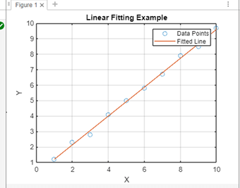

Based on the coefficients discovered during the linear fitting procedure, the fitted line is produced using the polyvalent function. Using the discovered coefficients, it evaluates the polynomial at the data points in x to get the corresponding fitted values of the dependent variable.

• The sample data points are fitted linearly using the polyfit function. We indicate that we wish to fit a first-degree polynomial, which translates to a straight line, by setting the third input to 1.
• The function yields the linear fit's coefficients, which stand for the best-fitting line's slope and y-intercept.

Applications:

Economic Analysis and Forecasting: GDP, inflation rates, and employment data are examples of the types of economic data that can be analyzed using linear fitting. Economists can foresee and predict future economic patterns with confidence by fitting linear models to historical data.

Physical sciences and engineering: Scientists and engineers use linear fitting to simulate physical phenomena like the decay of radioactive elements over time or the relationship between force and displacement in mechanical systems. Through the process of fitting linear models to experimental data, one can obtain important insights and forecast complicated system behavior.

Biomedical Research and Health Sciences: Data about medication dosages, patient reactions to treatments, and the course of diseases over time are all analyzed with the use of linear fitting in the field of biomedicine. Through the use of linear models to clinical data, researchers are able to determine therapy efficacy, forecast patient outcomes, and find relationships.

Market and Financial Analysis: When examining stock prices, market trends, and financial data, linear fitting is frequently used. Analysts can forecast future market movements, identify trends, and evaluate risk by fitting linear models to past stock market data.

Environmental Studies and Climate Analysis: When analyzing data on temperature fluctuations, ecological trends, and climate change, environmental scientists employ linear fitting. Researchers can evaluate the effects of human activity on the environment, forecast future climatic patterns, and suggest mitigation solutions by fitting linear models to environmental data.

Social Science and Education Research: Data on student performance, educational interventions, and social behavior are analyzed by social science and education researchers through the use of linear fitting. They can determine what influences a student's performance, evaluate the success of educational programs, and recommend policies based on data by fitting linear models to behavioral and educational data.