F-Zero in MATLAB

Introduction

FZero is a powerful optimization function in MATLAB that plays a crucial role in finding the roots of nonlinear equations. Whether you are a beginner or an experienced MATLAB user, understanding how to leverage FZero effectively can significantly enhance your ability to solve complex engineering and scientific problems.

In this comprehensive guide, we will delve into the intricacies of FZero, exploring its functionalities, applications, and best practices for implementation.

Getting Started with FZero:

Begin by introducing the basic syntax of FZero, highlighting its essential parameters. Explain the significance of the function to be solved, the initial guess, and any additional options that can be specified.

Supported Equations: Discuss the types of equations that FZero can handle, including single-variable and multi-variable equations. Provide examples to illustrate the diversity of problems that can be tackled using FZero.

Getting Started with FZero:

The fzero function in MATLAB is a powerful tool for finding the roots of nonlinear equations.

Syntax:

fun: The function handle represents the equation to be solved. This function should return a value close to zero when zero is called on it.

x0: The initial guess for the root.

Example:

Output: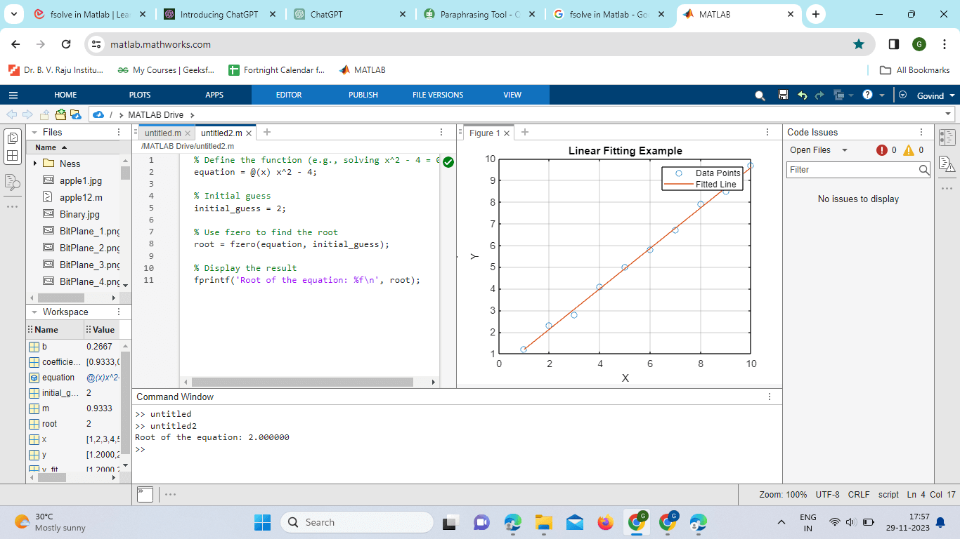

In this example, fzero attempts to find the root of the equation x^2 - 4 with an initial guess of 2. The result is the root of the equation.

Additional Options:

fzero provides additional optional parameters that allow users to customize the solving process:

Tolerance (tol): Specifies the tolerance for stopping the algorithm.

The default value is 1e-6.

% Set a custom tolerance

options = optimset('TolX', 1e-8);

root = zero(equation, initial_guess, options);

Maximum Iterations (maxiter): Sets the maximum number of iterations allowed. The default value is 100.

% Set a custom maximum number of iterations

options = optimset('MaxIter', 200);

root = zero(equation, initial_guess, options);

Supported Equations:

fzero is a versatile function capable of handling both single-variable and multi-variable equations. Let's explore the types of equations it can handle:

Single-Variable Equations:

% Single-variable equation: x^2 - 4 = 0

equation_single = @(x) x^2 - 4;

root_single = zero(equation_single, initial_guess);

Multi-Variable Equations:

% Multi-variable equation: y = x^2 + z

equation_multi = @(vars) vars(1)^2 + vars(2);

initial_guess_multi = [2, 1];

root_multi = zero(equation_multi, initial_guess_multi);

In the multi-variable case, the function should take a vector (vars in this example) as an input.

Diversity of Problems:

fzero can tackle a wide range of problems, including but not limited to:

Polynomial Equations: Solving equations involving polynomials, as shown in the examples above.

Trigonometric Equations: Finding roots of trigonometric equations such as sin(x) = 0.

Exponential Equations: Solving equations involving exponential functions, like 2^x - 8 = 0.

Applications of FZero:

Engineering Examples: Explore real-world engineering applications where FZero proves invaluable. This could include scenarios such as finding the roots of nonlinear equations representing electrical circuits, mechanical systems, or chemical processes.

Scientific Research: Discuss how FZero can be applied in scientific research, such as solving equations that arise in physics, biology, or environmental science. Provide specific examples to showcase the versatility of FZero across different domains.

Advanced Usage and Options:

Custom Objective Functions: Demonstrate how to use FZero with custom objective functions. This involves defining your functions to represent complex mathematical models or systems.

Tolerance and Iterations: Explain the importance of setting appropriate tolerance levels and understanding the iteration process. Showcase how adjusting these parameters can impact the accuracy and efficiency of the optimization.

Dealing with Constraints: Bound Constraints: Explore the concept of bound constraints and how they can be incorporated into FZero to limit the search space. Discuss scenarios where bound constraints are crucial and provide examples.

Nonlinear Constraints: Introduce the handling of nonlinear constraints within FZero, illustrating situations where these constraints are common in optimization problems.

Comparisons with Other MATLAB Optimization Functions:

FMinunc vs. FZero

Compare FZero with other optimization functions like FMinunc. Highlight the specific scenarios where FZero is more suitable and discuss the trade-offs between different optimization techniques.

Performance Considerations: Address the computational performance of FZero, considering factors such as convergence speed and memory usage. Provide tips for optimizing performance in large-scale problems.

Independence of Errors: The discrepancies between the observed and expected values, also known as residuals or errors, ought to be independent of one another. According to this presumption, the mistakes for one observation shouldn't affect the errors for subsequent observations.

Homoscedasticity: This suggests that at all levels of the independent variable, the variance of the residuals should stay constant. Stated otherwise, the residuals' distribution ought to remain constant across the independent variable's range.

Normalcy of Residuals: According to the normalcy assumption, the residuals need to be distributed normally. This indicates that a normal distribution with a zero mean should characterize the mistakes.

No Multicollinearity: Multicollinearity should not exist when there are several independent variables. Multicollinearity is the result of two or more separate.

Absence of Outliers or Important Points: The outcomes of the linear fit can be greatly impacted by outliers or important points. These data items have the potential to skew the calculated coefficients and, in turn, the model's overall fit.

• Although breaking these presumptions doesn't always mean the linear fit is wrong, it does have an impact on the precision and dependability of the findings.
• It is imperative to evaluate these assumptions and take appropriate action to rectify any infractions prior to implementing linear fitting in any analysis.
• In order to ensure the robustness of the linear fitting analysis, methods including residual analysis, diagnostics plots, and influential point identification can help evaluate and mitigate any violations of these assumptions.

Example:

Output: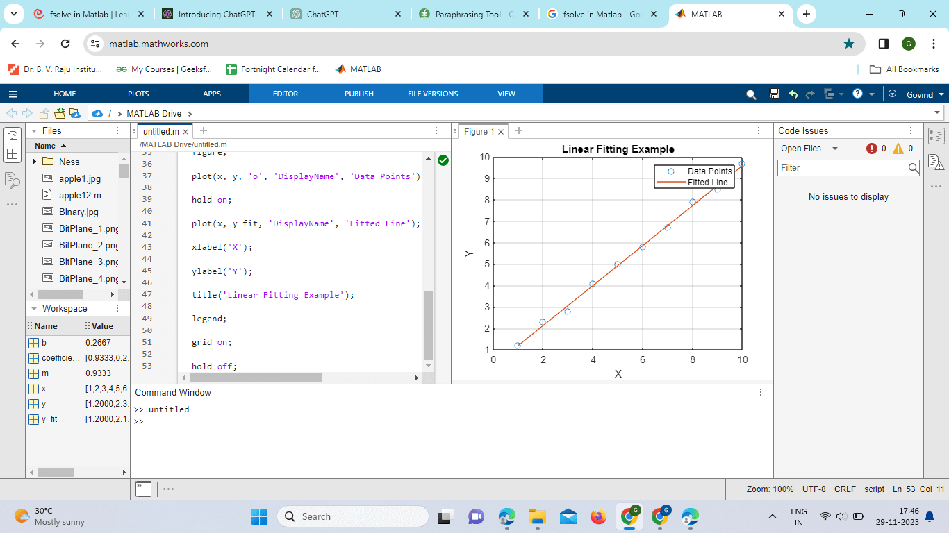

Based on the coefficients discovered during the linear fitting procedure, the fitted line is produced using the polyval function. Using the discovered coefficients, it evaluates the polynomial at the data points in x to get the corresponding fitted values of the dependent variable.

The sample data points are fitted linearly using the polyfit function. We indicate that we wish to fit a first-degree polynomial, which translates to a straight line, by setting the third input to 1. The function yields the linear fit's coefficients, which stand for the best-fitting line's slope and y-intercept.

Applications:

Economic Analysis and Forecasting: GDP, inflation rates, and employment data are examples of the types of economic data that can be analyzed using linear fitting. Economists can foresee and predict future economic patterns with confidence by fitting linear models to historical data.

Physical sciences and engineering: Scientists and engineers use linear fitting to simulate physical phenomena like the decay of radioactive elements over time or the relationship between force and displacement in mechanical systems. Through the process of fitting linear models to experimental data, one can obtain important insights and forecast complicated system behavior.

Biomedical Research and Health Sciences: Data about medication dosages, patient reactions to treatments, and the course of diseases over time are all analyzed with the use of linear fitting in the field of biomedicine. Through the use of linear models to clinical data, researchers are able to determine therapy efficacy, forecast patient outcomes, and find relationships.

Market and Financial Analysis: When examining stock prices, market trends, and financial data, linear fitting is frequently used. Analysts can forecast future market movements, identify trends, and evaluate risk by fitting linear models to past stock market data.

Environmental Studies and Climate Analysis: When analyzing data on temperature fluctuations, ecological trends, and climate change, environmental scientists employ linear fitting. Researchers can evaluate the effects of human activity on the environment, forecast future climatic patterns, and suggest mitigation solutions by fitting linear models to environmental data.

Social Science and Education Research: Data on student performance, educational interventions, and social behavior are analyzed by social science and education researchers through the use of linear fitting. They can determine what influences a student's performance, evaluate the success of educational programs, and recommend policies based on data by fitting linear models to behavioral and educational data.