Covariance in MATLAB

Introduction:

A Grasp the relationships between variables in a dataset requires a grasp of covariance in MATLAB. The amount that two random variables change together is measured by covariance. Positive covariance denotes a positive relationship between the variables, whilst negative covariance points to an inverse relationship. There is no linear relationship between the variables when the covariance value is zero.

MATLAB has various functions, such as cov and corr, for computing covariance. When calculating a dataset's covariance matrix, the cov function comes in handy.

Here is a quick overview of how to utilize MATLAB's cov function:

Syntax:

X: The input data, where a column and an observation by a row represent a variable.

C: The matrix of covariance. A matrix C is n by n symmetric if X has n columns. The covariance between the variables in columns i and j is represented by the element C(i,j).

Understanding Covariance Matrix

A thorough understanding of the connections between the variables in a dataset can be obtained from the covariance matrix that the cov function generates. Each element of the covariance matrix represents the covariance between two distinct variables. A linear relationship is shown by a zero value, a negative value shows a negative relationship and a positive value indicates a positive relationship.

• By identifying the variables that tend to vary together and those that are independent, an analysis of the covariance matrix can shed light on the dataset's structure.
• Furthermore, the strength of the correlations between the variables is indicated by the magnitude of the covariance values.

Analyzing the Findings

Understanding the underlying patterns and relationships within a dataset requires an interpretation of the covariance matrix. During the interpretation process, the following are some important things to remember:

Positive Covariance: When two variables have a positive covariance, they often tend to rise or fall together. This shows that the variables have a positive association and that, on average, when one variable rises, the other tends to follow suit.

Negative Covariance: On the other hand, a negative covariance indicates that the variables have an inverse connection. One variable tends to decrease when the other grows, and vice versa.

Zero Covariance: When there is no linear relationship between the variables, it is assumed that they are independent. It is crucial to remember that even in cases when two variables have zero covariance, they might still be connected in a nonlinear way.

How to Compute Correlation Coefficients

Although the covariance matrix offers insightful information, it needs to be standardized, which makes cross-dataset comparisons difficult. The corr function in MATLAB calculates the correlation matrix in order to remedy this. Correlation coefficients, which are normalized estimates of the associations between variables and range from -1 to 1, are contained in the correlation matrix.

Syntax:

X: Data matrix input. Each column and an observation by each row represent a variable.

R: Matrix of correlation. A matrix R is n by n symmetric if X has n columns. The correlation coefficient between the variables in matrix X's columns i and j is represented by the element R(i,j).

Making use of the corr function facilitates a more efficient comprehension of the direction and strength of linear correlations between variables.

Example:

Output: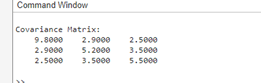

First, a sample dataset called X with three variables and five observations is created in this application. Next, we calculate the dataset's covariance matrix C using the cov function. Lastly, we show the computed covariance matrix C and the dataset X in the MATLAB command window.

Covariance Applications in MATLAB

In a number of disciplines, including statistics, finance, economics, and data science, knowing covariance in MATLAB is essential. Key uses of covariance in MATLAB include the following:

Portfolio analysis: Covariance is crucial to portfolio analysis in order to comprehend the connections between various assets. It aids in evaluating the advantages of diversification among various assets and optimizes the portfolio's overall risk and return profile.

Pattern Recognition: In jobs involving pattern recognition, such image and signal processing, covariance analysis is essential. One can find significant patterns and structures in the data by examining the covariance between various features.

Statistical modelling: Covariance is a key component of statistical modelling, which evaluates the correlations between various variables and creates prediction models based on patterns in the observed data.

Data Preprocessing: Covariance analysis assists with feature selection and dimensionality reduction, among other data preprocessing tasks. It helps to find features that are highly linked or duplicated, which may be eliminated to make the dataset.

Best Practices and Things to Think About

To guarantee accurate and significant findings when working with covariance in MATLAB, it is crucial to take into account a few recommended practices and safety measures:

Data Preprocessing: Before calculating the covariance, clean up and preprocess the data to remove any anomalies or discrepancies that could distort the findings.

Normalization: If required, normalize the data to guarantee that the variables are on the same scale. Variations in scales can have an impact on the covariance findings.

Caution in Interpretation: Since covariance only represents linear correlations between variables, care should be taken when interpreting its results. The covariance matrix might not be sufficient to express nonlinear interactions.

Data Visualization: To better understand the interactions between variables, visualize the covariance matrix and correlation matrix using heatmaps or other visualization approaches.

An essential statistical measure for comprehending the connections between the variables in a dataset is covariance.

• The covariance matrix may be easily computed in MATLAB using the cov function, the correlation matrix can be calculated, and normalized relationship measures can be obtained using the corr function.
• By utilizing these features and comprehending the ramifications of covariance analysis, users are able to make wise judgments, obtain insightful knowledge from their data, and create strong statistical models for a range of uses.
• MATLAB's robust computational capabilities make it an essential tool for

Example:

Output: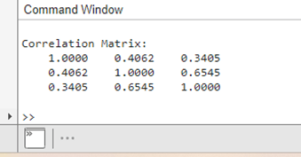

Explanation:

Sample Dataset:

The sample dataset X is represented by this matrix, where each column represents a variable and an observation by each row.

Covariance Matrix:

The covariance matrix shows how the variables in the dataset are correlated. Covariance between the variables in columns i and j is represented by each element of the matrix CovMatrix(i, j).

Correlation Matrix:

The correlation coefficients between the variables in the dataset are shown in the correlation matrix. The correlation between the variables in columns i and j is represented by each element of the CorrMatrix(i, j) matrix.

• These matrices shed light on the connections between the variables; the correlation matrix shows the normalized correlations, while the covariance matrix shows the raw relationships.
• In the matrices, values near zero denote a weak or nonexistent relationship; positive values indicate a positive relationship and negative values represent a negative relationship.

Visualizing Covariance Matrix as a Heatmap

Example:

Output: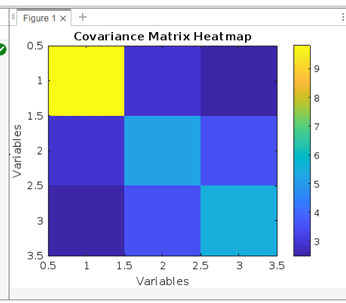

Explanation:

The covariance matrix C is visualized as a heatmap by the application. The covariance values between various pairs of variables in dataset X are displayed in a heatmap. Cooler hues denote negative covariance, while warmer hues show more positive covariance. Understanding the magnitude of the covariance values is made easier by the colour scale that the colorbar function provides.

• Plot type is indicated by the title 'Covariance Matrix Heatmap'; further context for the visualization is provided by the xlabel and ylabel functions, which label the variables on the axes.
• Users may easily spot patterns and relationships between the variables in the dataset by using this visualization, which offers an accessible approach to evaluate the covariance matrix.

Example:

Data Preprocessing and Covariance Calculation

Output: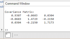

The software creates, centres, and adds noise to a random dataset before computing the covariance matrix for the preprocessed data. The centred data is displayed in the preprocessed dataset X_centered, and the covariances between the variables in the preprocessed dataset are displayed in the covariance matrix C.