Curve Fitting in MATLAB

Introduction:

Curve fitting stands as a cornerstone of data analysis and modeling in a myriad of scientific and engineering domains. It encompasses the task of identifying a mathematical function that best corresponds to a given set of data points. MATLAB, renowned for its prowess in numerical computing, offers a diverse array of tools that facilitate curve fitting with unparalleled ease and adaptability.

This guide endeavors to furnish a comprehensive exploration of curve fitting within the MATLAB environment, encompassing fundamental concepts, diverse curve fitting techniques, and practical implementations for elucidating their real-world applications.

• At its core, curve fitting involves constructing a mathematical curve that accurately represents a sequence of data points.
• The primary objective is to discern a model that encapsulates the underlying trends in the data, thereby enabling prediction, interpolation, or extrapolation.
• MATLAB, serving as a potent tool, empowers researchers and engineers to analyze and interpret intricate datasets with exceptional efficiency.

Basic Concepts in MATLAB

Prior to delving into the intricacies of curve fitting techniques within MATLAB, it is imperative to grasp a few foundational concepts:

Data Preparation: Organize the data into arrays or matrices within MATLAB, ensuring that the data is in a suitable format for the specific curve fitting technique employed.

Function Evaluation: Leverage MATLAB's diverse built-in functions to evaluate mathematical expressions and execute operations on arrays and matrices.

Data Plotting: Harness MATLAB's plotting capabilities to visualize the data in both pre-and post-curve fitting. This aids in comprehending the data's behavior and the efficacy of the selected curve-fitting technique.

Types of Curve Fitting Techniques

Linear Curve Fitting

Linear curve fitting involves fitting a linear model to the data, assuming a linear relationship between the independent and dependent variables. MATLAB provides potent tools for executing linear regression and least squares fitting, such as the poly fit and fitlm functions.

A simple and widely used method for determining the best-fitting linear connection between two variables is linear curve fitting. The goal of the linear curve fitting approach is to approximate the relationship, represented in the following manner, as a straight line between the independent variable (x) and the dependent variable (y):

Where y-intercept (b) is represented by y-intercept (b) and slope (m) is the slope of the line. Finding the values of m and b that minimize the sum of squared differences between the dependent variable's observed and anticipated values is the method.

When there is a linear relationship between the variables being considered, linear curve fitting is frequently utilized. It is frequently used in many different domains, including the social sciences, engineering, physics, and economics.

Example of Linear Curve Fitting:

Suppose you have a set of data points, and you want to fit a linear model to the data. Using the method of least squares, you can find the best-fitting line that minimizes the sum of the squared vertical distances between the observed data points and the corresponding points on the line.

Here's an example:

Suppose you have the following data points:

X=1,2,3,4,5

Y=2,3.5,3.8,5,4.5

Using linear curve fitting, you can find the best-fitting line that represents the relationship between x and y.

• This line can be represented as y=mx+b, where m is the slope and b is the y-intercept.
• The goal is to find the values of m and b that minimize the sum of the squared differences between the observed and predicted values of y for each x.

Polynomial Curve Fitting

Polynomial curve fitting is a method used to find the best-fitting polynomial function that represents the relationship between two variables. Unlike linear curve fitting, polynomial curve fitting allows for the fitting of curves that are not necessarily straight lines.

The general form of a polynomial curve of degree n is given by:

the coefficients of the polynomial, and n is the degree of the polynomial.

The goal of polynomial curve fitting is to determine the coefficients of the polynomial that minimize the difference between the observed data points and the values predicted by the polynomial function. This is commonly achieved using the method of least squares, which minimizes the sum of the squared differences between the observed and predicted values.

Example:

Let's consider an example of polynomial curve fitting. Suppose we have the following data points:

X=1,2,3,4,5

Y=:2,3.5,3.8,5,4.5

We want to find a polynomial function that best fits these data points. Let's try to fit a polynomial of degree 2,

which has the form:

Nonlinear Curve Fitting

When a linear or polynomial function is unable to explain the data, nonlinear curve fitting adequately is a useful technique for determining the best-fitting model that depicts the connection between variables. Nonlinear curve fitting, in contrast to linear or polynomial curve fitting, entails fitting a model with nonlinear parameters.

• A nonlinear model's general form can be more intricate and incorporate a variety of functions, including power, logarithmic, exponential, and trigonometric functions.
• Finding the model's parameters that minimize the discrepancy between the values predicted by the model and the observed data points is the aim of nonlinear curve fitting. Typically, optimization methods that reduce the total squared discrepancies between the observed

Example of Nonlinear Curve Fitting:

Suppose we have the following data points representing an exponential relationship:

x:1,2,3,4,5

y:2.5,3.5,6.2,8.9,12.4

We can fit an exponential model of the form y=aebx to the data points. The goal is to find the values of a and b that minimize the difference between the observed and predicted values of y for each x. We can use optimization techniques, such as the Levenberg-Marquardt algorithm, to find the best-fitting parameters for the exponential model.

Examples Linear Regression

Output: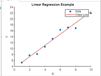

Explanation:

Simple linear regression example, where a linear relationship is fitted to noisy data, and the result is visualized for analysis. Adjustments can be made to the data generation process or the degree of the polynomial fit, depending on specific requirements.

Example 2: Nonlinear Curve Fitting

Output: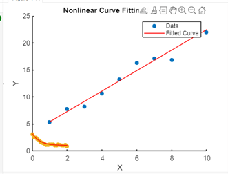

• Always visually assess the data prior to curve fitting to gain insights into its behavior. Select an appropriate curve fitting technique based on the data characteristics and underlying model.
• Regularly validate the fitted model by comparing it with the original data and conducting statistical analyses.
• Consider the trade-off between model complexity and overfitting to prevent the model from capturing noise instead of the underlying trend.
• Document the entire curve fitting process, encompassing the chosen technique, parameters, and any assumptions made during the analysis.

MATLAB offers potent tools for executing diverse curve-fitting operations, allowing users to analyze and interpret intricate datasets with unparalleled efficiency. By harnessing MATLAB's built-in functions and the Curve Fitting Toolbox, researchers and engineers can extract invaluable insights from data, make precise predictions, and construct reliable models for real-world applications. An in-depth comprehension of the fundamental concepts and best practices for curve fitting in MATLAB proves vital in making well-informed decisions and obtaining meaningful results in data analysis and modeling tasks.

Curve Fitting Toolbox

The MATLAB Curve Fitting Toolbox is a powerful resource designed for conducting a variety of curve-fitting tasks. Accessible both through the MATLAB command window and a user-friendly graphical interface, this toolbox offers an array of indispensable features:

Curve Fitting Functions: A diverse selection of functions, including those for linear, nonlinear, and custom equation fitting, provides ample flexibility. The toolbox accommodates various models, such as polynomials, exponentials, logarithmic, and power functions.

Data Preprocessing: With capabilities for data smoothing, outlier removal, and handling missing data, users can ensure the accuracy and reliability of the fitting process.

Model Assessment: The toolbox facilitates the thorough evaluation of fitted models by providing crucial statistical measures like R-squared values, residuals, and confidence intervals. This feature aids in assessing the model's goodness of fit and overall reliability.

Model Comparison and Selection: Tools for comparing multiple models based on criteria such as the Akaike information criterion (AIC), Bayesian information criterion (BIC), and cross-validation assist users in selecting the most suitable model.

Visualization: Various plotting functions, including scatter plots, line plots, error plots, and confidence interval plots, enable users to visualize both data and fitted models effectively. This visualization capability enhances the understanding of the relationship between data points and the fitted curves.

Optimization and Customization: Users can exercise control over the fitting process by customizing fitting options and constraints to cater to specific requirements. Moreover, the toolbox provides optimization algorithms that refine parameter estimation, enhancing the accuracy of the fitted models.

The Curve Fitting Toolbox within MATLAB effectively streamlines the curve fitting process, empowering users to conduct comprehensive data analysis and interpretation with its wide range of tools and functionalities.