Matlab Remainder

Introduction:

MATLAB, which stands for MATrix LABoratory, is a robust numerical computing environment that finds extensive application in a wide range of industries, such as data analysis, finance, physics, and engineering. Remainders are essential to many MATLAB computational tasks, from simple arithmetic operations to more intricate algorithms. We will examine remainders in MATLAB, go into their concept, and provide you real-world examples to help you understand how they might be used.

Basic Arithmetic Operations and Remainders:

Division and Remainders: In MATLAB, the Remainder of a division operation can be obtained using the 'rem' function. This function is particularly useful when you need to find the remainder after dividing one number by another.

dividend = 17;

divisor = 5;

remainder = rem(dividend, divisor);

disp(['The remainder of ', num2str(dividend), ' divided by ', num2str(divisor), ' is ', num2str(remainder)]);

This basic example demonstrates how to use the 'rem' function to compute the Remainder of 17 divided by 5.

Modulus Function: MATLAB also provides the 'mod' function, which can be used to find the Remainder similar to 'rem.' However, there is a subtle difference between the two functions, and understanding when to use each is essential.

dividend = 17;

divisor = 5;

remainder = mod(dividend, divisor);

disp(['The remainder of ', num2str(dividend), ' divided by ', num2str(divisor), ' is ', num2str(remainder)]);

We'll explore the differences between 'rem' and 'mod' and discuss scenarios where one might be more suitable than the other.

÷4, the Quotient is 3 with a Remainder of 1 because 4×3+1=134×3+1=13.

Let's deeper into each of these elements:

Dividend: The Dividend is the numerical quantity subjected to division. It signifies the total amount that we aim to distribute into equal parts during the division process.

Example: In the division problem 12 ÷ 3, the Dividend is 12.

Divisor: The Divisor is the number by which the Dividend is divided. It denotes the quantity of parts into which the Dividend is partitioned during the division operation.

Example: In the division problem 12 ÷ 3, the Divisor is 3.

Quotient: The Quotient is the outcome of the division operation. It signifies the factor by which the Divisor is multiplied to obtain a product that is equal to or approximates the Dividend.

Example: In 12 ÷ 3, the Quotient is 4 since 3 × 4 = 12.

Remainder: When the product of Divisor * Quotient is not precisely equal to the Dividend, a remainder exists. The Remainder indicates the amount that remains after completing the division process.

Example: In 13 ÷ 4, the Quotient is 3 with a Remainder of 1 because 4 × 3 + 1 = 13.

• Understanding these four quantities is fundamental to grasping the concept of division in mathematics.
• They provide a clear structure for expressing the process of sharing or distributing a quantity into equal parts.
• In practical terms, division is a fundamental arithmetic operation used in various real-world scenarios, from splitting resources among a group of people to calculating proportions and ratios in diverse fields such as finance, engineering, and science.

Applications of Remainders in MATLAB:

Checking for Even or Odd Numbers: Remainders are often used to determine whether a given number is even or odd. In MATLAB, this can be achieved by checking the Remainder when dividing by 2.

number = 24;

if rem(number, 2) == 0

disp([num2str(number), ' is an even number.']);

else

disp([num2str(number), ' is an odd number.']);

end

We'll explore how this concept can be extended to solve more complex problems and optimize algorithms.

Implementing Clock Arithmetic: Remainders play a significant role in clock arithmetic, where values wrap around after reaching a certain limit. MATLAB leverages remainder to simulate cyclic behavior, as seen in applications like timekeeping and signal processing.

hours = 27;

max_hours = 24;

corrected_hours = rem(hours, max_hours);

disp(['The corrected hours are: ', num2str(corrected_hours)]);

Implementation:

Output: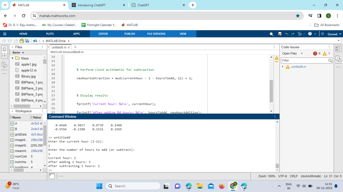

Explanation:

Function Declaration:

function clockArithmetic

The program starts by defining a MATLAB function named clock arithmetic.

User Input:

current hour = input('Enter the current hour (1-12): ');

hoursToAdd = input('Enter the number of hours to add (or subtract): ');

The program prompts the user to input the current hour on a 12-hour clock (1-12) and the number of hours to add or subtract.

Clock Arithmetic for Addition:

newHourAddition = mod(current hour - 1 + hoursToAdd, 12) + 1;

It uses the mod function to perform clock arithmetic for addition. The (current hour - 1 + hoursToAdd) part calculates the theoretical hour after addition, and mod(..., 12) ensures it wraps around to stay within the 12-hour clock range. The + 1 adjusts it back to the 1-12 range.

Clock Arithmetic for Subtraction:

newHourSubtraction = mod(current hour - 1 - hours to add, 12) + 1;

Similarly, it performs clock arithmetic for subtraction. The (current hour - 1 - hoursToAdd) part calculates the theoretical hour after subtraction, and the rest of the logic ensures it wraps around within the 12-hour clock range.

Display Results:

Finally, the program displays the current hour, the new hour after addition, and the new hour after subtraction using fprintf.

Advanced Topics in MATLAB Remainders:

Polynomial Remainder Theorem:

MATLAB's polynomial toolbox allows users to perform polynomial division and obtain remainders using the 'polyder' and 'polyval' functions.

We'll explore the Polynomial Remainder Theorem and how it relates to more advanced applications in MATLAB.

Implementation:

Output: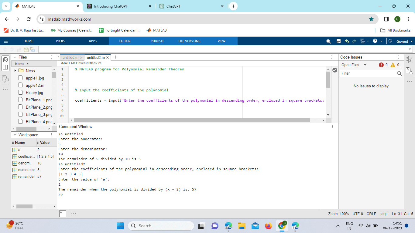

Signal Processing and FFT:

In signal processing, remainders are encountered when working with discrete signals and applying the Fast Fourier Transform (FFT). Understanding how to interpret and handle remainders is crucial for accurate signal analysis.

signal = randn(1, 1024); % a random signal of length 1024

fft_result = fft(signal);

We'll demonstrate how remainders come into play during signal processing tasks and discuss best practices for handling them.

Example:

Program for Signal Processing and FFT

Output: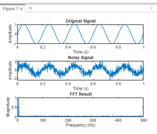

Explanation:

Generate a Signal: A sinusoidal signal with a frequency of 5 Hz is generated.

Add Noise: To replicate a real-world situation, Gaussian noise is applied to the signal.

Execute FFT: The frequency components of the noisy signal are analyzed by applying the Fast Fourier Transform.

Plot Results: To display the original signal, the noisy signal, and the FFT result, three subplots are made.

Show Dominant Frequency: The application determines and shows the signal's dominant frequency.

• Remainders are a key notion in MATLAB that extends beyond basic arithmetic operations.
• They have uses in many different domains, ranging from basic operations like determining if a given number is even or odd to more complex ones like signal processing and polynomial mathematics.
• Through proficiency with remainders in MATLAB, users can improve the accuracy and efficiency of their numerical calculations.
• This comprehensive guide serves as a valuable resource for both beginners and experienced MATLAB users, providing insights and practical examples to deepen their understanding of this essential mathematical concept.

Implementation:

Output: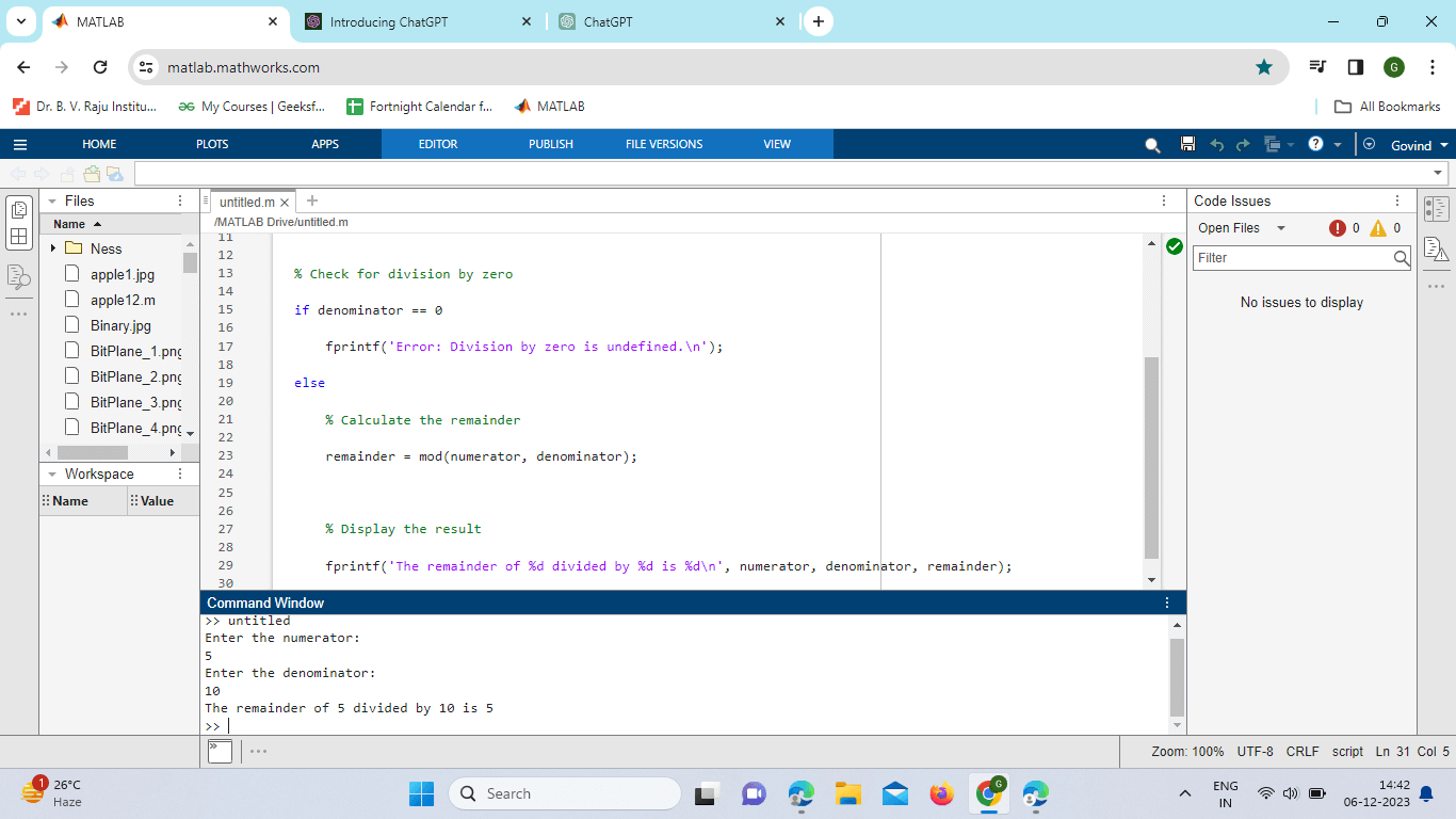

Explanation:

Check for Division by Zero: The program checks if the denominator is zero. Division by zero is undefined in mathematics, so if the denominator is zero, the program displays an error message and stops. Otherwise, it proceeds to the other block.

Calculate Remainder: The program calculates the Remainder of the division of the numerator by the denominator using the mod function.