Matlab fft()

MATLAB's FFT Function

MATLAB, a powerful tool widely used in scientific and engineering fields, offers numerous functions for signal processing and analysis. One of the fundamental functions in MATLAB's arsenal is fft(), which stands for Fast Fourier Transform. The FFT is a mathematical algorithm utilized to transform a signal from the time domain to the frequency domain, allowing for efficient analysis of the signal's frequency components.

What is the FFT?

One popular method for calculating the Discrete Fourier Transform (DFT) and its inverse is the Fast Fourier Transform. When compared to traditional DFT, it significantly lowers computational complexity, which makes it appropriate for huge data sets and real-time applications. By breaking down a signal into its individual frequencies, the FFT offers important insights into the spectral content of the signal.

Fourier Transform:The Fourier Transform, or FT, is a mathematical instrument that breaks down a signal into its individual frequencies. It shows the amplitude and phase of each frequency that is present in the signal by representing the signal in terms of its frequency components.

Discrete Fourier Transform (DFT): This discrete Fourier transform is used to calculate a discrete sequence or signal's frequency-domain representation. It computes a series of complex numbers that represent the signal in the frequency domain from a finite sequence of evenly spaced function samples.

FFT Algorithm: The FFT algorithm is a highly effective DFT implementation that can calculate the DFT considerably quicker than the conventional DFT approach, particularly for lengthy sequences. When N is the number of samples in the sequence, it lowers the number of operations needed to compute the DFT from O(N2) to O(NlogN).

Applications: Signal processing, image processing, audio processing, communications, and scientific computing are just a few of the domains in which the FFT finds extensive use. Spectrum analysis, filtering, convolution, correlation, and many more tasks are among the many uses for it.

Properties: The linearity, time-shift, frequency-shift, convolution, and correlation properties of the DFT are all preserved by the FFT. It makes it possible to compute these operations in the frequency domain efficiently.

Syntax of fft() in MATLAB:

Where:

X is the input signal, typically a vector representing discrete time-domain samples.

Y is the output, representing the discrete Fourier transform of the input signal.

Syntax Variations:

This function computes the Discrete Fourier Transform (DFT) of signal f using the Fast Fourier Transform (FFT) algorithm.

Returns the frequency domain signal F.

Specifying the Number of Points:

Computes the DFT of signal f using the FFT algorithm with n points.

Returns the frequency domain signal F with n points. By default, F has the same size as f.

Specifying Dimension:

Computes the DFT of signal f using the FFT algorithm along the dimension specified by dim.

Returns the frequency domain signal F along the dimension dim.

Additional Notes:

f: Input signal or array.

n: Number of points for the DFT. By default, it is the size of f.

dim: Dimension along which the FFT is applied. This is optional and useful when dealing with multidimensional arrays. If not specified, FFT is applied along the first non-singleton dimension.

Example Usage:

% Basic u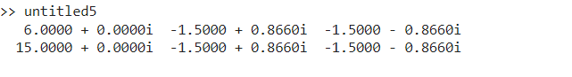sage
f = [1, 2, 3, 4];
F = fft(f); % Computes FFT of 'f'

% Specifying the number of points
n = 8;
F = fft(f, n); % Computes FFT of 'f' with 'n' points

% Specifying dimension
A = [1, 2, 3; 4, 5, 6];
F = fft(A, [], 2); % Computes FFT along the second dimension of 'A'
Disp(F);

Output:

Basic Usage:

Using fft() in MATLAB is straightforward. Pass the signal you want to analyze as an input argument to the function.

Example:

Fs = 1000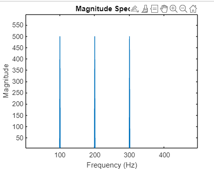; % Sampling frequency (Hz) 
t = 0:1/Fs:1-1/Fs; % Time vector 
x = sin(2*pi*100*t) + sin(2*pi*200*t) + sin(2*pi*300*t); % Example signal 
Y = fft(x); % Compute FFT
f = linspace(0, Fs, length(Y)); % Frequency vector
Y_mag = abs(Y); % Magnitude spectrum
plot(f(1:length(Y)/2), Y_mag(1:length(Y)/2)) % Plot half of the spectrum
xlabel('Frequency (Hz)')
ylabel('Magnitude')
title('Magnitude Spectrum')

Output:

In this example, x represents a synthetic signal composed of three sinusoidal components at frequencies 100 Hz, 200 Hz, and 300 Hz. By applying fft(), we obtain Y, which contains information about the amplitudes and phases of these frequency components.

Need to Know

If f is a Vector: The function fft(f) computes the Fourier transform of vector f, producing F as the result.

If f is a Matrix, fft(f) processes each column of matrix f separately, calculating the Fourier transform for each column. The resulting output F would be the Fourier transform of each column.

If f is a Multidimensional Array, fft(f) treats the values along the first non-singleton array dimension as vectors. It computes the Fourier transform for each vector along this dimension. The resulting output F will retain the array structure, with Fourier transforms computed along the appropriate dimension.

Interpreting the Output:

The output of fft() yields a complex-valued vector Y representing the discrete Fourier transform of the input signal x. To visualize the spectral content, we often plot the magnitude or power spectrum. This can be achieved using abs() to compute the magnitude of the complex values in Y.

Example:

f = (0:leng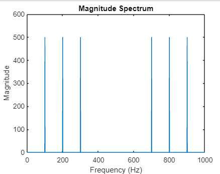th(Y)-1)*Fs/length(Y);   % Frequency vector
plot(f, abs(Y))
xlabel('Frequency (Hz)')
ylabel('Magnitude')
title('Magnitude Spectrum')

Output:

This code plots the magnitude spectrum of the FFT output versus frequency. It helps visualize the amplitudes of different frequency components present in the signal.

Advanced Usage and Options:

While the basic usage of fft() suffices for many applications.

MATLAB offers additional options to tailor the FFT computation to specific needs:

Specifying FFT Length: By default, MATLAB's fft() computes the FFT using the smallest power of 2 that is greater than or equal to the length of the input signal.

However, users can specify the FFT length explicitly using the syntax Y = fft(X, N), where N is the desired FFT length.

Windowing: Applying a window function to the input signal before computing the FFT can reduce spectral leakage and improve frequency resolution, especially when analyzing finite-duration signals.

MATLAB provides various windowing functions, such as Hamming, Hanning, and Blackman.
Users can apply windowing using element-wise multiplication (.*) before calling fft().

Two-Sided vs. One-Sided Spectrum: By default, MATLAB's FFT function computes a two-sided spectrum, which includes both positive and negative frequencies.

However, for real-valued signals, the spectrum is symmetric, and analyzing only the positive frequencies can suffice, effectively halving the computational burden.
Users can achieve this by considering only the first half of the FFT output.

Frequency Binning: When analyzing the FFT output, it's essential to understand the frequency resolution, which is determined by the sampling frequency and FFT length.

MATLAB provides functions like fftshift() to rearrange the FFT output to center the zero-frequency component and fftfreq() to compute the corresponding frequency bins.

Example:

Fs = 1000;                         % Sampling frequency (Hz)
t = 0:1/Fs:1-1/Fs;                 % Time vector
x = sin(2*pi*100*t) + sin(2*pi*200*t) + sin(2*pi*300*t);   % Example signal

% Compute FFT with explicit length and apply Hanning window
N = 1024;                          % FFT length
windowed_x = x .* hann(length(x)); % Apply Hanning window
Y = fft(windowed_x, N);            % Compute FFT with specified length

% Plot one-sided magnitude spectrum
f = (0:N/2)*Fs/N;                  % Frequency vector
plot(f, abs(Y(1:N/2+1)))
xlabel('Frequency (Hz)')
ylabel('Magnitude')
title('One-Sided Magnitude Spectrum')

Output:

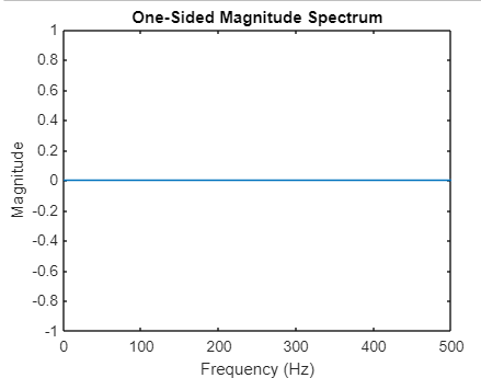
In this example, we explicitly specify the FFT length as 1024 and apply a Hanning window to the input signal before computing the FFT. The resulting one-sided magnitude spectrum provides a clearer representation of the signal's frequency content.

Example:

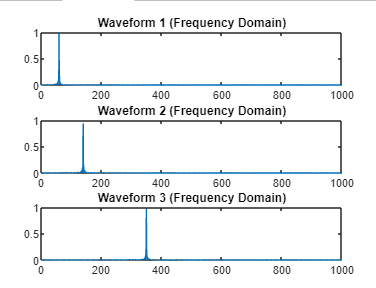
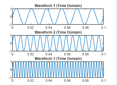
% Define sampling parameters
Fs = 2000;          % Sampling frequency
Ts = 1/Fs;          % Sampling period
Ls = 3000;          % Length of signal
t = (0:Ls-1)*Ts;    % Time vector

% Generate sinusoidal waves with different frequencies
r1 = sin(2*pi*60*t);    % Waveform with frequency 60 Hz
r2 = sin(2*pi*140*t);   % Waveform with frequency 140 Hz
r3 = sin(2*pi*350*t);   % Waveform with frequency 350 Hz

% Plot each sinusoidal wave in the time domain
figure;
for k = 1:3
    subplot(3,1,k);
   % plot(t(1:200), eval(['r', num2str(k)](1:200))); % Plot first 200 samples
plot(t(1:200), r{k}(1:200)); % Plot first 200 samples

    title(['Waveform ', num2str(k), ' (Time Domain)']);
end

% Compute FFT for each waveform and plot in the frequency domain
np = 2^nextpow2(Ls);    % Next power of 2 for FFT
d = 2;                  % Perform FFT along the rows (dimension 2)
F = fft([r1; r2; r3], np, d);   % Compute FFT for the matrix of waveforms
PS2 = abs(F/Ls);        % Compute two-sided spectrum
PS1 = PS2(:,1:np/2+1); % Extract single-sided spectrum
PS1(:,2:end-1) = 2*PS1(:,2:end-1);  % Duplicate amplitudes (except DC and Nyquist) for single-sided spectrum

% Plot single-sided amplitude spectrum in frequency domain
figure;
for k = 1:3
    subplot(3,1,k);
    plot(0:(Fs/np):(Fs/2-Fs/np), PS1(k,1:np/2)); % Plot frequency content
    title(['Waveform ', num2str(k), ' (Frequency Domain)']);
end

Output:

This version simplifies variable names and provides clearer comments for each section of the code. It generates three sinusoidal waves, plots them in the time domain, computes their FFT, and plots the single-sided amplitude spectrum in the frequency domain for each waveform.

MATLAB's fft() function, coupled with its advanced options, empowers users to perform in-depth spectral analysis on signals, facilitating a deeper understanding of their characteristics.

By leveraging features like windowing, frequency binning, and one-sided spectrum computation, MATLAB users can extract meaningful insights from their data, enabling informed decision-making across various domains.

Next Topic#

← prev next →