Heaviside in Matlab

Introduction:

The Heaviside step function often denoted as H(t) or u(t), is a fundamental mathematical tool that finds wide-ranging applications in engineering, physics, and various scientific disciplines. Named after the British mathematician Oliver Heaviside, this step function captures the essence of sudden transitions or step changes in mathematical models.

In this comprehensive exploration, we delve into the intricacies of the Heaviside step function, focusing on its definition, properties, applications, and practical implementation using MATLAB.

Definition and Properties:

The Heaviside step function is defined as follows:

0 & \text{if } t < 0 \\ 
1 & \text{if } t \geq 0\
end{cases} \] At \(t = 0\),

The function undergoes an instantaneous change from 0 to 1, creating a step-like transition.

This definition makes the Heaviside step function a valuable tool for modeling systems with abrupt changes or sudden inputs.

The properties of the Heaviside step function include: -

Unit Step: The Heaviside function is often referred to as the unit step function, representing a step of unit height at \(t = 0\).

Symmetry:\(H(t) = 1 - H(-t)\) reflects the symmetry of the function about the y-axis. -

Integral Representation: The Heaviside function is closely related to the unit impulse function (\(\delta(t)\)), and its integral yields the unit ramp function (\(r(t)\)). - Derivative: The derivative of the Heaviside function is the Dirac delta function (\(\delta(t)\)), a distribution widely used in mathematical physics.

Advanced Usage and Techniques:

MATLAB offers various techniques for advanced usage of the Heaviside function. Engineers and researchers often encounter scenarios where the Heaviside function needs to be manipulated or combined with other functions for more complex modeling.

Piecewise Functions:

The `piecewise` function in MATLAB enables the definition of piecewise functions, allowing users to express functions with different behaviors in distinct intervals. The Heaviside function is often integrated into piecewise functions to represent varied conditions.

Example:

% Define 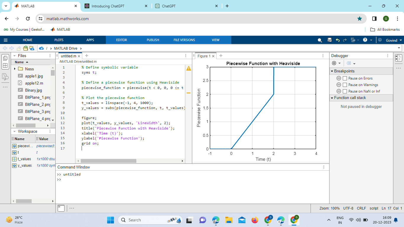symbolic Variable

syms t;

% Define a piecewise function using Heaviside

piecewise_function = piecewise(t < 0, 0, 0 <= t < 2, t, t >= 2, 2 + heaviside(t - 2));

% Plot the piecewise function

t_values = linspace(-1, 4, 1000);

y_values = subs(piecewise_function, t, t_values);

figure;
plot(t_values, y_values, 'LineWidth', 2);

title('Piecewise Function with Heaviside');
xlabel('Time (t)');

ylabel('Piecewise Function');
grid on;

Output:

Explanation:

Symbolic Variable: t is defined as a symbolic variable to allow symbolic expressions.

Piecewise Function Definition: The piecewise function is used to define a piecewise function. In this example:

Plotting: The program generates values for the piecewise function over a range of t_values and plots the result.

Visualization: The plot shows the piecewise function with different behaviors in different intervals, with a step-like change at 0=2t=2 due to the Heaviside function.

This program illustrates how the piecewise function, along with the Heaviside function, can be used to express complex conditions and create functions that change their behavior at specific points. The piecewise function is a useful tool in mathematical modeling, allowing you to represent different cases within a single expression.

Convolution:

The convolution operation is frequently used in signal processing. MATLAB provides the `conv` function, which can be used in conjunction with the Heaviside function to convolve two signals.

Consider the convolution of two-step functions:

Example:

t = -5:0.1:5; 

u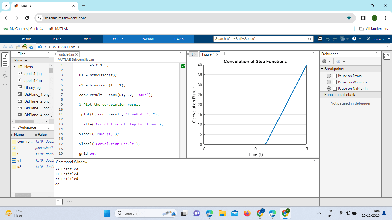1 = heaviside(t); 

u2 = heaviside(t - 1);
 
conv_result = conv(u1, u2, 'same'); 

% Plot the convolution result 

plot(t, conv_result, 'LineWidth', 2); 

title('Convolution of Step Functions'); 

xlabel('Time (t)'); 

ylabel('Convolution Result'); 

grid on;

Output:

Explanation:

Time Vector (t): A time vector t is created ranging from -5 to 5 with a step of 0.1. This vector represents the time axis for our signals.

Heaviside Step Functions (u1 and u2): Two Heaviside step functions, u1 and u2, are defined. u1 is the step function that turns on at t = 0, and u2 is similar but delayed by 1 unit of time.

Convolution (conv_result): The convolution of u1 and u2 is calculated using the conv function with the 'same' option. This option ensures that the result has the same length as the input vectors.

Plotting the Convolution Result: The convolution result is plotted against the time vector t. The 'LineWidth' 2 parameters are used to make the plot lines thicker for better visibility.

Plot Labels and Title: Labels for the x-axis, y-axis and a title are set for the plot.

Grid On: The grid is turned on to aid in visualizing the plot.

Convolution with Heaviside Function:

Convolution is a mathematical operation that combines two functions to produce a third. The Heaviside function is often involved in convolution operations. Let's explore convolution using the Heaviside function:

t = -5:0.1:5;
u1 = Heaviside(t);
u2 = heaviside(t - 1);

conv_result = conv(u1, u2, 'same');

% Plot the convolution result
figure;
subplot(3, 1, 1);
plot(t, u1, 'LineWidth', 2);
title('Heaviside Function 1');
xlabel('Time (t)');
ylabel('H(t)');

subplot(3, 1, 2);
plot(t, u2, 'LineWidth', 2);
title('Heaviside Function 2');
xlabel('Time (t)');
ylabel('H(t-1)');

subplot(3, 1, 3);
plot(t, conv_result, 'LineWidth', 2);
title('Convolution Result');
xlabel('Time (t)');
ylabel('Convolution');

Output: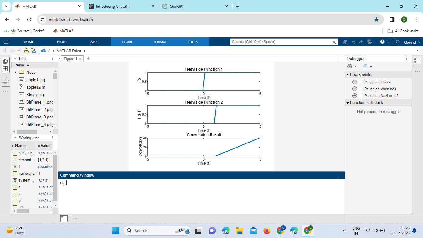

Explanation:

This part creates a figure with three subplots to visualize:u1 in the first subplot and u2 in the second subplot.

The convolution results in the third subplot. The code generates plots to show how two-step functions (u1 and u2) change over time and their convolution result, which represents the combined effect of these functions. The convolution result should look like a triangular pulse due to the convolution of two Heaviside functions.

Symbolic Toolbox Integration:

For users with the Symbolic Math Toolbox, MATLAB allows for the symbolic representation of mathematical expressions, including the Heaviside function. This feature facilitates symbolic computations and algebraic manipulations involving the Heaviside function.

Example:

% Clear s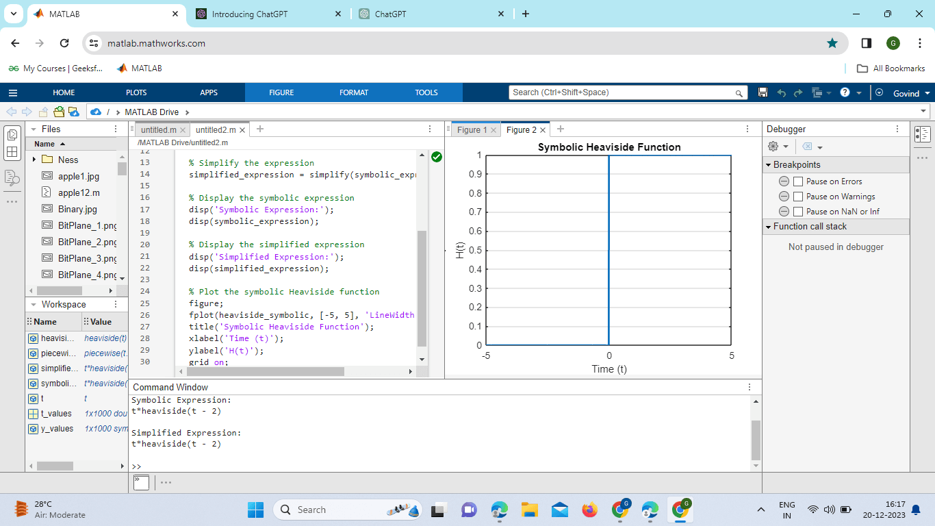ymbolic variables (if any)
clear sym;
% Define symbolic Variable
syms t;
% Define a symbolic Heaviside function
heaviside_symbolic = heaviside(t);
% Define a symbolic expression involving the Heaviside function
symbolic_expression = t * Heaviside(t - 2);
% Simplify the Expression
simplified_expression = simplify(symbolic_expression);
% Display the symbolic Expression
disp('Symbolic Expression:');
disp(symbolic_expression);
% Display the simplified Expression
disp('Simplified Expression:');
disp(simplified_expression);
% Plot the symbolic Heaviside function
figure;
plot(heaviside_symbolic, [-5, 5], 'LineWidth', 2);
title('Symbolic Heaviside Function');
xlabel('Time (t)');
ylabel('H(t)');

Output:

Explanation:

Symbolic Variable (t): A symbolic variable t is defined using syms.

Symbolic Heaviside Function (heaviside_symbolic): The symbolic Heaviside function is defined using Heaviside (t).

Symbolic Expression Involving Heaviside (symbolic_expression): A symbolic expression involving the Heaviside function is defined as t⋅H(t-2)).

Simplify the Expression (simplified_expression): The simplify function is used to simplify the symbolic Expression.

Display Symbolic and Simplified Expressions: The symbolic and simplified expressions are displayed.

Plot Symbolic Heaviside Function: The symbolic Heaviside function is plotted over a range of t values.

Practical Examples in Control Systems:

The Heaviside step function finds prominent applications in control systems, where it is utilized to model the response of a system to sudden changes or inputs.

Consider a simple example of a first-order system responding to a step input:

Numera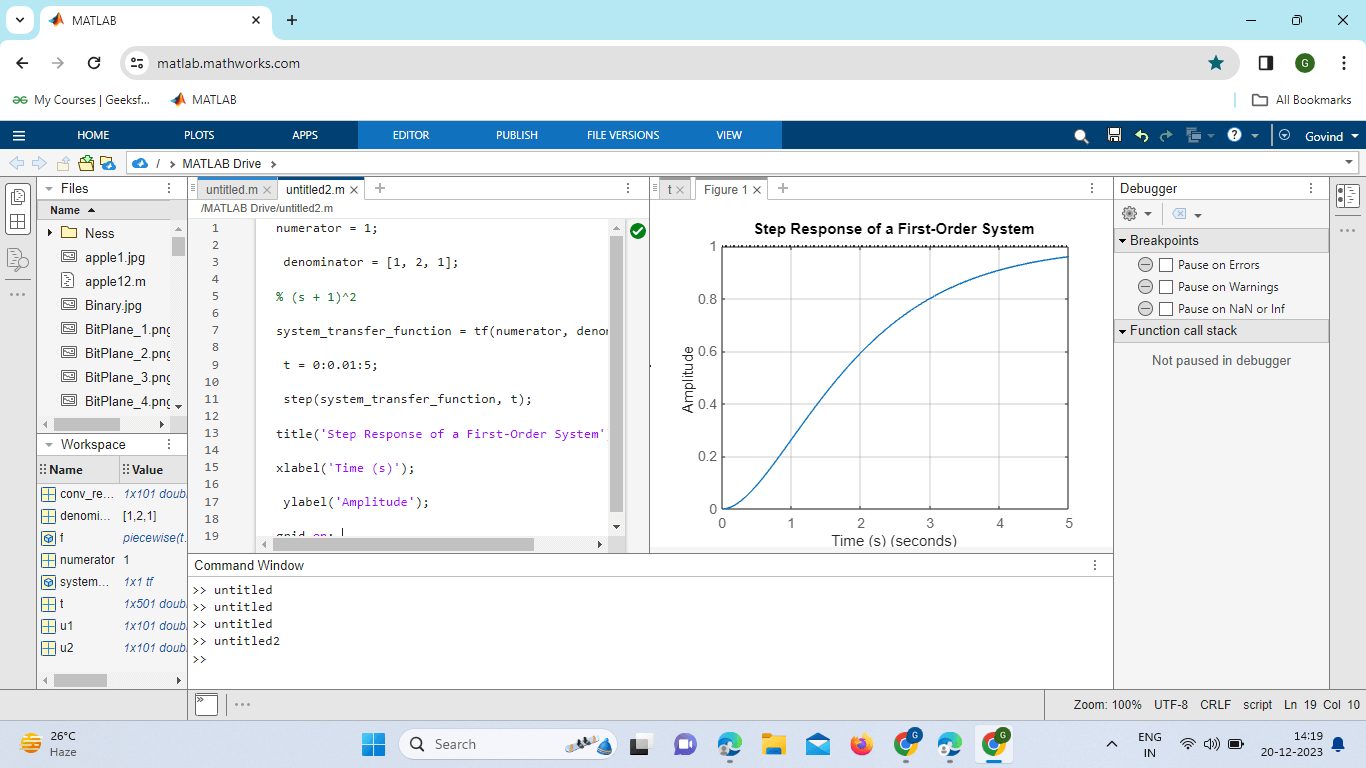tor=1;

denominator = [1, 2, 1]; 

% (s + 1)^2 

system_transfer_function = tf(numerator, denominator); 

t = 0:0.01:5;
 
step(system_transfer_function, t); 

title('Step Response of a First-Order System'); 

xlabel('Time (s)'); 

ylabel('Amplitude');
 
grid on;

Output:

Explanation:

In this example, a first-order system's step response is simulated using the transfer function and the `step` function in MATLAB. The Heaviside function is implicitly involved in computing the system's response to the step input, highlighting its importance in control systems.

Transfer Function Coefficients: The numerator is set to 1, and the denominator coefficients represent the characteristic equation 2(s+1)2 of a first-order system. The transfer function is 2H(s)=(s+1)21 .

Transfer Function Object (system_transfer_function): The tf function creates a transfer function object using the specified numerator and denominator coefficients.

Time Vector (t): A time vector t is defined from 0 to 5 with a step of 0.01 seconds. This vector represents the time axis for the simulation.

System Response Simulation (step): The step function simulates the step response of the system represented by system_transfer_function over the specified time vector t.

Plot Title and Labels: The plot is given a title, and labels are set for the x-axis (Time) and y-axis (Amplitude).

Numerical Considerations: W

When dealing with the Heaviside function or step-like inputs, numerical simulations may encounter issues due to the finite precision of computer arithmetic. It is crucial to choose an appropriate time step (ODE solver time step) to accurately capture the behavior of the system, especially around the points of abrupt changes represented by the Heaviside function. In some cases, users may need to experiment with different solver options or adaptive time-stepping strategies to improve the accuracy of the simulation results.

Example:

% Define 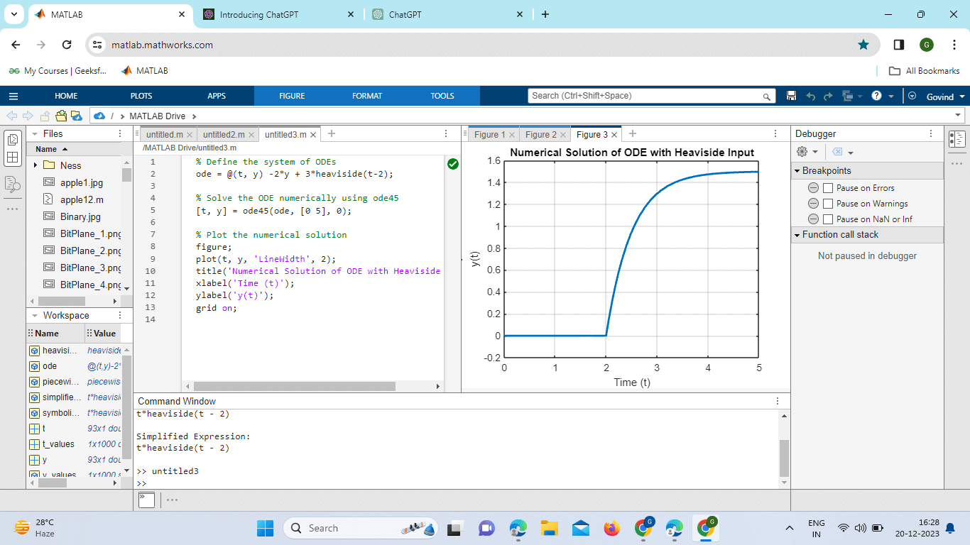the system of ODEs

ode = @(t, y) -2*y + 3*heaviside(t-2);

% Solve the ODE numerically using ode45

[t, y] = ode45(ode, [0 5], 0);

% Plot the numerical Solution
figure;
plot(t, y, 'LineWidth', 2);

title('Numerical Solution of ODE with Heaviside Input');

xlabel('Time (t)');

ylabel('y(t)');

grid on;

Output:

Explanation:

System of ODEs (ode): A system of ordinary differential equations (ODEs) is defined. In this example, it represents study =-2y+3u(t-2), where u(t-2) is the Heaviside step function.

Numerical Solution (ode45): The ode45 solver is used to numerically solve the ODE over the time interval [0, 5].

Plotting the Numerical Solution: The numerical Solution is plotted over time using the plot function.

Plot Title and Labels: The plot is given a title, and labels are set for the x-axis (Time) and y-axis

Handling Numerical Stability:

When working with numerical simulations involving the Heaviside function, it's crucial to consider numerical stability. Small-time steps may lead to numerical artifacts. Applying a suitable numerical integration method, such as the ode45 solver, can enhance accuracy.

Example:

% Define 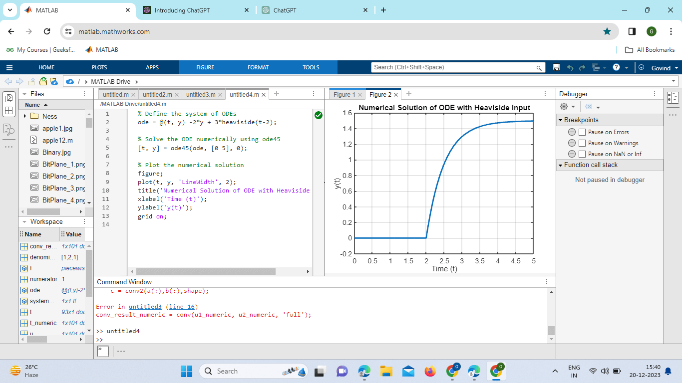the system of ODEs
ode = @(t, y) -2*y + 3*heaviside(t-2);

% Solve the ODE numerically using ode45
[t, y] = ode45(ode, [0 5], 0);

% Plot the numerical Solution
figure;
plot(t, y, 'LineWidth', 2);
title('Numerical Solution of ODE with Heaviside Input');
xlabel('Time (t)');
ylabel('y(t)');
grid on;

Output:

This script uses the ode45 solver to numerically solve a differential equation with a Heaviside input numerically, ensuring better stability over a range of time steps.

The Heaviside step function in MATLAB proves to be a versatile and powerful tool, extending its applications from basic signal processing to symbolic manipulation, convolution, control system analysis, and differential equations. As demonstrated in these advanced examples, its seamless integration into MATLAB facilitates a wide array of mathematical and engineering simulations. Understanding and leveraging the capabilities of the Heaviside function in MATLAB opens the door to diverse applications in research, engineering, and education.

Engineering Applications:

The Heaviside step function is a staple in engineering applications, playing a vital role in modeling various phenomena. In electrical engineering, it is used to represent the response of circuits to sudden changes in input voltages or currents. In mechanical engineering, it can model the behavior of systems subjected to abrupt forces or displacements. Its application extends to telecommunications, control systems, and beyond.

Engineering Applications of the Heaviside Step Function:

The Heaviside step function is a fundamental tool in engineering, finding widespread applications across various disciplines. Its ability to represent sudden changes or step inputs makes it indispensable in modeling dynamic systems. Here are some key engineering applications:

Electrical Engineering: Circuit Analysis: In electrical engineering, the Heaviside function is used to model and analyze the response of circuits to sudden changes in input voltages or currents. It helps characterize the transient behavior of circuits during switching events or sudden power changes.

Mechanical Engineering: System Dynamics: In mechanical engineering, the Heaviside step function is employed to model the behavior of mechanical systems subjected to abrupt forces, displacements, or changes in loading conditions. It is particularly useful in studying the transient response of structures and mechanisms.

Telecommunications: Signal Processing: The Heaviside function is extensively used in telecommunications for signal processing applications. It plays a crucial role in modeling and analyzing the response of communication systems to sudden changes in signal characteristics, such as amplitude or frequency.

Control Systems: Controller Design: In control systems engineering, the Heaviside step function is a key element in representing step inputs or disturbances. It is used to analyze and design controllers that can respond effectively to sudden changes in the system's reference or disturbance inputs.

Civil Engineering: Structural Analysis: Civil engineers use the Heaviside function to model the response of structures to sudden loads or seismic events. It helps in predicting the dynamic behavior of buildings, bridges, and other infrastructure components.

Aerospace Engineering: Vehicle Dynamics: Aerospace engineers apply the Heaviside function to model the dynamic response of aircraft and spacecraft to sudden changes in control inputs or external forces. It aids in understanding the transient behavior of aerospace systems.

Biomedical Engineering: Physiological Modeling: In biomedical engineering, the Heaviside step function can be employed to model physiological responses to sudden stimuli. For example, it might be used in modeling the neural response to a sudden external stimulus.

Environmental Engineering: Environmental Impact Modeling: Engineers studying the environmental impact of sudden events, such as pollutant releases or industrial accidents, can use the Heaviside step function to model the immediate response of ecosystems. The Heaviside step function is a powerful mathematical tool with diverse applications across scientific and engineering disciplines.

MATLAB's seamless integration of the Heaviside function allows for efficient modeling and analysis of systems with sudden changes or step inputs.
From basic usage to advanced techniques, the versatility of the Heaviside step function makes it an indispensable asset for researchers, engineers, and students alike.
This comprehensive exploration has aimed to shed light on the various facets of the Heaviside step function, providing both theoretical insights and practical guidance for its effective use in MATLAB.

Next TopicKalman Filter Matlab

← prev next →