Simpson Method

The Simpson is a numerical integration method that was given by Thomas Simpson and so was named the Simpson method. Although there are certain rules of Simpson, the most basic are the two rules of Simpson which are:

• Simpson's 1 rule: It is known as Simpson's 1/3 rule
• Simpson's 2 rule: It is known as Simpson's 3/8 rule

In this section, we will discuss both of these Simpson's rules and will also implement the example code of both the rules.

Simpson's 1/3 Rule

It is also known as Simpson's Rule where the rule says: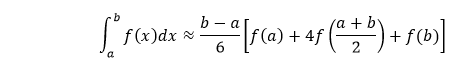

where f(x) is the integrand, a is the lower limit, and b is the upper limit of integration in the expression.

Quadratic Interpolation

Replace the integrand f(x) with a quadratic polynomial P(x) which is the parabola and takes same values of limits a and b as f(x). It also calculates m = (a + b)/2 as in f(x). Hence, on using Lagrange Polynomial Interpolation and integration by substitution we get,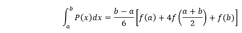

Then use step size h=(b-a)/2 and then it can be written as: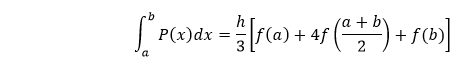

As it is h/3, i.e., 1/3 factor, we call it the Simpson's rule as Simpson's 1/3 rule.

The Simpson's rule can be derived via the below graph where we have approximated the integrated f(x) by P(x), which is the quadratic interpolant.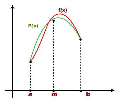

Numerical Example

For solving a numerical, we need to use the Simpson's rule i.e.

Numerical: Evaluate logx dx within limit 4 to 5.2.

Solution:

Step 1: Choose a value in which the intervals will be divided, i.e., the value of n. So, for the given expression, first, we will divide the interval into six equal parts as the number of intervals should be even.

Step 2: Calculate the value of h = (b - a)/2

Step 3: Evaluate and calculate the values of x₀ to x_n. Consider y = f(x) and calculate the values of y₀ to y_n for x₀ to x_n. Here, we get the following data: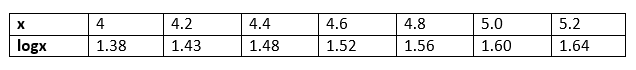

Step 3: Put the values in the method and then we can calculate approximate value of integral using above formula:

= h/3[( 1.38 + 1.64) + 4 * (1.43 + 1.52 +

1.60 ) +2 *(1.48 + 1.56)]

= 1.84

Hence the approximation of the above integral is 1.827 using Simpson's 1/3 rule.

Program Implementation for Simpson's 1/3 Rule

Below is the program code implementation in C for the Simpson's 1/3 rule:

The output of the above code is shown below: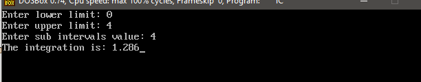

Simpson 3/8 Rule

It is the second rule of Simpson and also similar to Simpson 1/3 rule but with a difference. The difference between the 1/3 and 3/8 rule is that in the Simpson 3/8 rule, the interpolant is a cubic polynomial. The Simpson 3/8 rule says: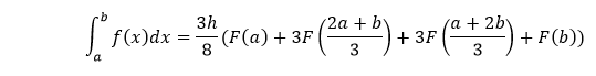

where f(x) is the integrand and h is the size of the interval which is calculated as h = (b - a)/n, and n is the interval limit here.

Now, let's see the program implementation to understand the logic behind the Simpson 3/8 rule.

Program to implement Simpson 3/8 rule

Below is the program code implementation in C++:

The output of the above code is shown below: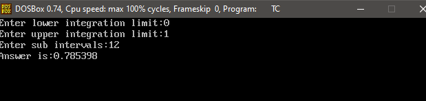

Other than these discussed two rules of Simpson, there is third rule existence that is used in the naval architecture and ship stability estimation. However, in the general approach, it has no importance.