ANOVA in the Microsoft Excel

ANOVA, or "Analysis of Variance", is defined as the single as well as the two-factor method which can be efficiently used to perform the null hypothesis test. It sates that if the particular performed test would be PASSED for Null Hypothesis if and only if all the population values are exactly equal to each other respectively.

If any or at least one of the particular values is a bit different from other values, then the null hypothesis would get FAILED. So, to perform the ANOVA Test in Microsoft Excel, with the help of the given "Data menu tab", we need to go to the "Data Analysis option", which is present just under the Analysis section. From there, we will select the ANOVA - Single Factor among other listed ANOVA Tests. After that, we will select the input and output range per our requirements. And once we encounter the output or the outcomes, it would be easy to conclude if we can consider or reject the respective amount of the data based on comparing F and the F-Critical values.If the F < F-Critical, then we can consider the Null Hypothesis to be PASSED, and else we will consider it FAILED.

Moreover, the "ANOVA" in the respective Microsoft Excel is primarily considered the statistical method that can efficiently test the difference between two or more means.

Why make use of the ANOVA in Microsoft Excel?

It was assumed that in Microsoft Excel, the particular "ANOVA", which is a one-way analysis of variance, can be effectively used in order to determine the various factors of those mean, whether they are statistically significant or not, in which the mean square usually denotes out the variation between the sample means, which means that it simply test out the null hypothesis.

How to find out the Anova Add-ins in Microsoft Excel?

It was known that in the respective Microsoft Excel, we could easily add the add-ins by downloading it from the internet or purchasing the specific add-ins. Nowadays, we can easily find many downloadable add-ins on the internet.

The respective Microsoft Excel comes with add-ins named such as the Data analyzer, Data Solver etc. And few COM-add-ins can efficiently add in Microsoft Excel, like the Power Pivot, etc..

Various steps that can be used to add Anova add-ins in the Microsoft Excel

In Microsoft Excel, add-ins are constantly groped under the "DATA menu" menu by default, and Microsoft Excel does not have add-ins. The data menu will get appear on the screen respectively.

Moving further, we can order to add add-ins to Microsoft Excel, and for that, we must follow the steps mentioned below very carefully.

Step 1: First of all, in Microsoft Excel, we need to go to theFile menu.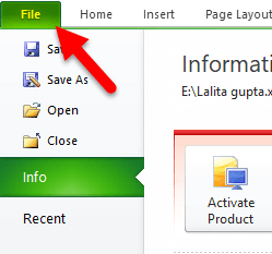

Step 2: Now, we will choose the optionfield (where in the older version, we can find the same option called as. "EXCEL OPTION"), as we can see in the below-attached screenshot.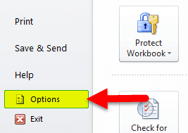

Step 3: TheExcel optionsdialogue box window will appear.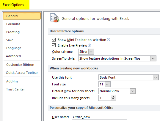

Step 4: We can see the add-ins columns on the left side of the pane. Click on theadd-ins option.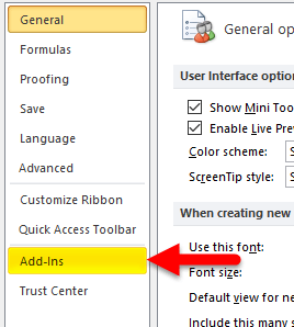

Step 5: And once we will click on the respective add-ins option, it shows a list of add-ins; and the very first part depicts the active Add-ins are installed that can be effectively used in the excel, and similarly the second part depicts out the Inactive Add-ins which are no more longer available in the Microsoft Excel.

Step 6: And at the bottom of the respective window, we will find the "manage option ", in which we can effectively manage the add-ins over here.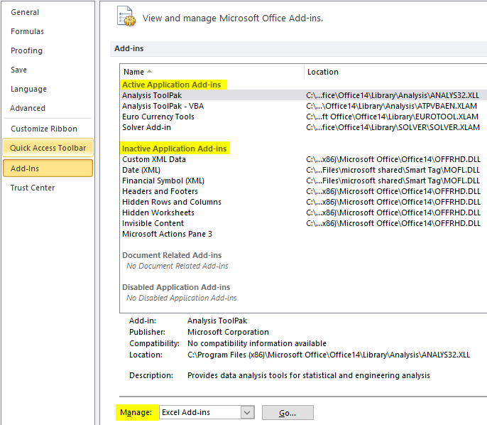

Adding the Excel- Add-ins

It was known that in Microsoft Excel, in the particular "Manageoption", we have the availability of the add-ins option such as the Microsoft Excel add-ins, COM add-ins, Action, XML expansion packs, and also the Disabled Items respectively.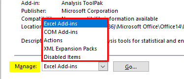

Now on moving further, let us see how to add excel-add with the help of the following mentioned steps:

Step 1: First, we will click on the active add-in to add it to Microsoft excel.

Step 2: After that, we will see how to activate the respective Excel add-in in Microsoft Excel, shown in the first part, with the help of the attached screenshot.

Step 3: Then, after that, we will be selecting out the first add-insAnalysis ToolPack respectively.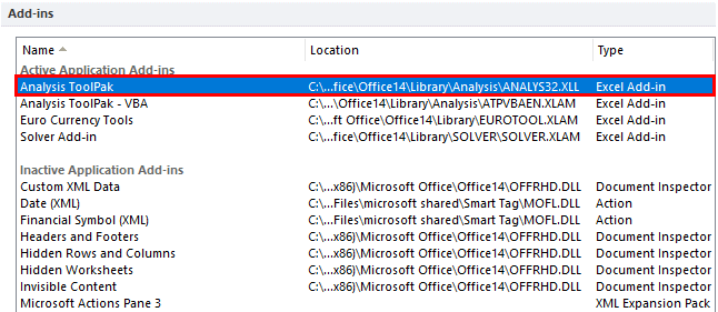

Step: 4 At the bottom, we will see that the manager drop-down box is available, and from there, we will select theExcel-add-insand then move on to the "Gooption "respectively, as seen in the below-attached figure.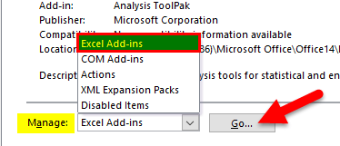

Step 5: Soon after performing the above, we will get theAdd-Ins window.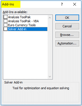

Step 6: Now, the particular analysis tool pack will contain out the set of add-ins that will allow us to choose it.

Step 7: After that, we will be encountered with the various available options, such as the Analysis Tool Pak-VBA, Analysis Tool Pack Euro Currency Tools, as well as the Solver Add-in, respectively.

Step 8: Now, after that, we will perform the Checkmarks toall the add-ins and then click on the "OK button" so that the particular selected add-ins will be displayed in the data menu effectively, as seen in the below-attached screenshot.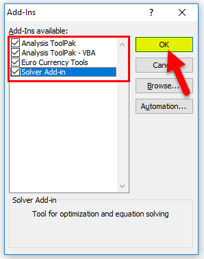

Step 9: Now, after adding out the add-ins, now we needs to check or make sure whether the add-ins has been added to the data menu or not.

Step 10: From the Excel ribbon bar click on the "Datamenu", and here you will find that all respective add-ins are added.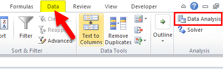

Now, after performing all the above, we can see that in the particular data tabData Analysishas been added under the analysis group, which are highlighted in Red color.

How to make Use of the ANOVA in Microsoft Excel?

ANOVA in Microsoft excel is termed to be a very simple as well as an easy-to-use concept which can be clearly understood by beginners (individual programmers or employees) too, now besides all these, let us see the working of the excel ANOVA single factor built-in tool with the help of different examples.

# Example: 1 Excel Anova

In this particular example, we will see how to effectively apply the respective Excel ANOVA single factor with the help of the example below.

Now let us consider the example below, showing students' marks scored on each subject, as shown in the screenshot below.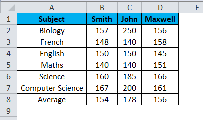

Now we are checking out the student's significantly different marks, with the help of the ANOVA tool, by just following the steps below.

Step 1: First of all, we will move to theDATAmenu options and then will click on theDATA ANALYSIS, as shown in the below-attached screenshot.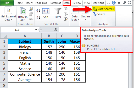

Step 2: The analysis dialogue box appears on our screen.

Step 3: You will get the various available list of the analysis tools. Look for the ANOVA- Single-factor tool.

Step 4: Click on theANOVA: Single-factortool and then clickthe "OK button", as clearly seen in the screenshot below.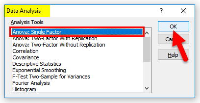

Step 5: Soon after performing the above steps, the ANOVA: Single-factor dialogue box will appear, as clearly depicted in the screenshot below.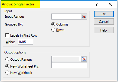

Step 6: Next, we will click on the input range box to select the range, which is the $B$1:$D$7.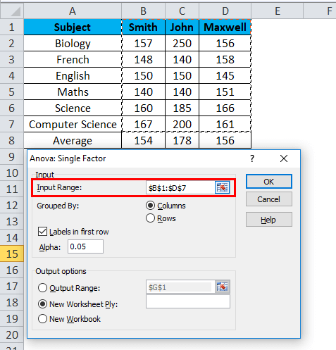

Step 8: As from the screenshot above attached, we have selected the ranges along with the student name in order to get the exact output.

Step 9: And now, the input range has been selected out. After that, we will ensure thatColumnCheckbox is selected.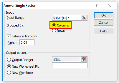

Step 10: Now, in this step, we want to select the output range where our output needs to be displayed efficiently.

Step 11: After that, we will click on the output range box and select the output cell in the respective worksheet, as shown in the figure below.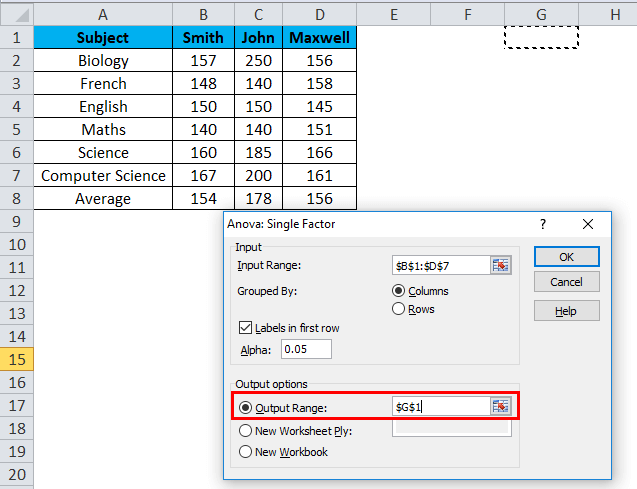

Step 12: From the above screenshot, it has been seen that we have selected the output range cell as G1, in which the output will be displayed.

Step 13: Then we will ensure that Labels in the first-rowCheckbox are selected, and then we will click onthe OK button.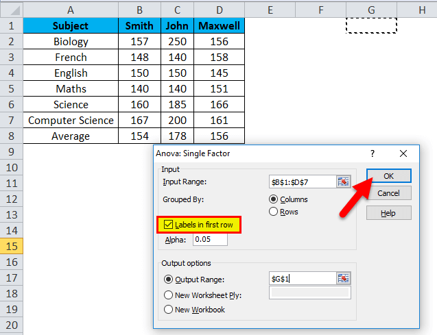

Step 14: We will get the below output as follows.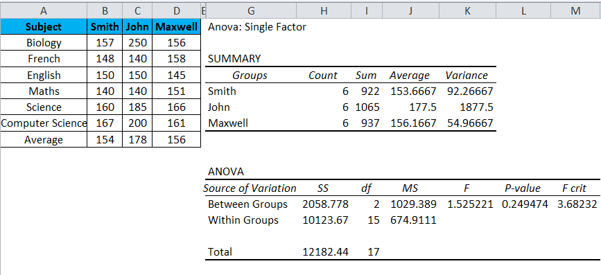

And the above-attached screenshot will show the summary part and Anova, where the summary part contains the Group Name, No of Count, Sum, Average and Variance, and the Anova shows the list of summaries where we need to check out theF value as well as the F Crit value.

Things to Remember

One needs to remember the following point while workings on the ANOVA in Microsoft Excel:

1. The Microsoft Excel ANOVA tool will efficiently work if we have correct input or if we end up with inaccurate data.
2. And it should ensure that the first variance value must be much smaller in comparison to the second variance value in order to get the accurate Value of F respectively.