Logical Functions in Excel

"Logical functions are used to compare more than one condition or multiple conditions. It returns the result as TRUE or FALSE by evaluating the arguments."

These functions are used for calculating the result and help to elect any one of the given data. Based on the requirement, the contents in the cell are evaluated using the respective logical condition. Here in this tutorial, the types of Logical Functions used are,

as it is used to evaluate the result.

AND Function

The AND function tests single or multiple conditions. It returns the value true if all the values evaluate to true and return false if any one of the value evaluates to false. This condition evaluates more than one condition, accepting 255 conditions called arguments. Arguments include expressions, constants, arrays, and cell references.

Syntax

=AND (logical 1, [logical 2]...)

Arguments

logical 1- The condition or value to be evaluated, which is called the first logical condition

logical 2- The condition or value to be evaluated, which is called the second logical condition

Similarly, the arguments are evaluated in the respective serial wise based on the number of conditions.

Some of the examples using AND function are as follows,

Example 1: Evaluate the given data using AND condition

To evaluate the data using certain conditions, the steps to be followed are

Enter the data in the worksheet namely A1:A5
Here, the data present in A1:A5 are calculated as greater than 1 and lesser than 100.
Select a new cell and enter the formula as = AND (A1:A5>1, A1:A5<100). Press Enter.
The result will be displayed as either TRUE or FALSE in the selected cell.

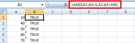
The result in the worksheet will be displayed as TRUE as the condition evaluates to true.

IF and AND Function

The IF and AND functions are used together for multiple conditions.

Example 2: Evaluate the given data using IF and AND function

Enter the data in the worksheet, namely A1:A2
Here the data present in A1:A2, the value in A1 are displayed if A1<A2 and A1<100. If the condition is false, it displays the message "The value is out of range".
Select a new cell and enter the formula as = IF (AND (A1<A2, A1<100), A1, "The value is out of range"). Press Enter.
The result will be displayed as either the value present in cell A1 or "The value is out of range"

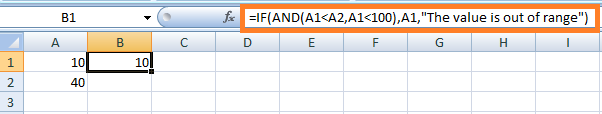
The result in the worksheet will be displayed as 10, where the arguments satisfy the condition.

The two cell values are compared using IF and AND functions.

Example 3: Evaluate the given data using IF and AND function

Enter the data in the worksheet, namely A1
Here, the data in A1 and the value in A1 are displayed if A1>1 and A1<100. If the condition is false, it displays the message "The value is out of range".
Select a new cell and enter the formula as = IF (AND (A1>1, A1<100), A1, "The value is out of range"). Press Enter.
The result will be displayed as either the value present in cell A1 or "The value is out of range"

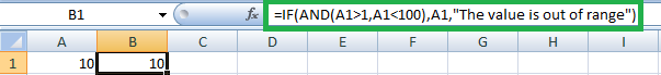
The result in the worksheet will be displayed as 10, where the arguments are true.

Example 4: Evaluate the given data using the argument "Approved" or "Denied"

Enter the data in the worksheet, namely A1:A5
Here, the data present in A1:A5, the argument is if A1>1 and A1<100. If the condition is false, it displays the message "Denied," or if it is true, it displays the message "Approved."
Select a new cell and enter the formula as = IF (AND (A1>1, A1<100), "Approved", "Denied"). Press Enter.
The result will be either "Approved" or "Denied".

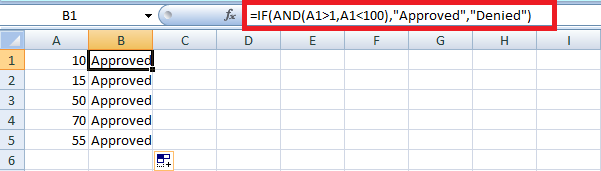
The result in the worksheet will be displayed as "Approved" as the argument satisfies the condition.

In example 4, the value of a single cell is compared with the arguments.

Note: The AND function is not case sensitive, and wildcard is not supported. The # VALUE will display if no logical values exist in the given function.

OR Function

The OR function returns the result as True if any arguments evaluate to true and return False if all the arguments evaluate to False. It acts on multiple testing conditions. It is combined with AND function and IF condition based on the requirement.

Syntax

Parameters

Logical 1- It represents the first condition to be evaluated

Logical 2- It represents the second condition to be evaluated.

The OR function syntax accepts up to 255 conditions entered as arguments. Arguments such as expressions, cell references, constant and logical expressions, and arrays are accepted.

The examples of the OR function are explained below follows,

Example 1: Evaluate the given data using OR function

To evaluate the data using OR condition, the steps to be followed are:

Enter the data in the worksheet, namely A1.
Here, the data present in A1 are calculated, which is greater than 1 and lesser than 100.
Select a new cell and enter the formula as = OR (A1>1, A1<100). Press Enter.
The result will be displayed as either TRUE or FALSE in the selected cell.

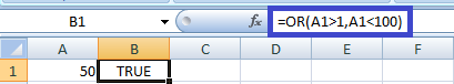
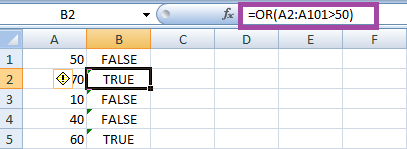
In the worksheet, the result will be displayed as TRUE where the arguments present in the condition evaluate to true. In example 1, the arguments are based on a single cell.

Example 2: Evaluate the data present in the cell using the OR function for multiple cells.

Enter the data in the worksheet, namely A1:A2
The data present in A1 and A2 are calculated based on the condition if the value present in A1 and A2 is greater than the specified value
Select a new cell and enter the formula as =IF (OR (A1>70, B1>60), "Pass", "Fail")
Press Enter. The result will be displayed in the selected cell.

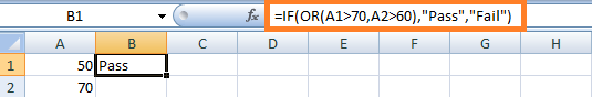
The first argument present in the condition is evaluated as false, and the second argument in the condition is evaluated as true. Here one of the arguments is evaluated to be true. Hence the result will be displayed as Pass.

Example 3: Evaluate the data using the array condition.

Enter the data in the worksheet, namely A1:A5
The array function is used to calculate the large data set.
Select a new cell and enter the formula as =OR (A1:A100>70)
Press Enter. The result will be displayed in the selected cell if the argument is evaluated to be true.
The result will be displayed in cell B1. To get the result for the remaining cells, drag the formula toward cell 101. The multiple cells are compared using the condition. In the OR condition, the argument is specified as A1:A101, hence any value entered in the cell range from A1:A101 which is greater than 50, the result will be displayed as TRUE, and if the condition fails, FALSE will be generated.

Example 4: Evaluate the given data using IF and OR function

Enter the data in the worksheet, namely A1:A3
Here the data present in A1:A3, the value in A3 are displayed if A1>10 and A1<A2. If the condition is false, it displays the message "The value is out of range".
Select a new cell and enter the formula as = IF (OR (A1>10, A1<A2), A3, "The value is out of range"). Press Enter.
The result will be displayed as either value present in cell A3 or "The value is out of range".

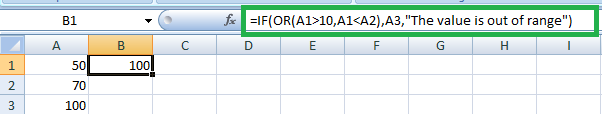
The result will be displayed as 100 as the arguments are considered true. Here IF and OR condition is used for multiple conditions.

Example 5: Evaluate the given data using IF and OR function

Step 1: Enter the data in the worksheet, namely A1

Step 2: Here, the data in A1 and the value in A1 are displayed if A1>50 and A1<70. If the condition is false, it displays the message "The value is out of range".

Step 3: Select a new cell and enter the formula as = IF (OR (A1>50, A1<70), A1, "The value is out of range"). Press Enter.

Step 4: The result will be displayed as either the value present in cell A1 or "The value is out of range".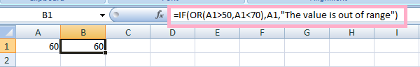

The arguments present in the condition are evaluated to be true. Hence the value present in cell A1 is displayed as a result.

NOT Function

NOT is one of the logical functions which return the reversed logical value. An inbuilt function in Excel is used along with the formula based on the requirement.

Syntax

Parameters

Logical value- An expression is used to evaluate either TRUE or FALSE

As described before, the NOT function reverses the value of the argument. Therefore, if the logical value is TRUE, the result will be false, and if the logical value is FALSE, the result will be TRUE.

Some of the examples of NOT function are as follows,

Example 1: Evaluate the given data using the NOT function

To evaluate the data using the NOT condition, the steps to be followed are

Step 1: Enter the data in the worksheet, namely A1:A4

Step 2: Here, the data present in A1:A4 are calculated, which greater than 75 is.

Step 3: Select a new cell and enter the formula as = NOT (A1>75). Press Enter.

Step 4: The result will be displayed as either TRUE or FALSE in the selected cell. To get the result for the remaining cells, drag the formula toward cell A4.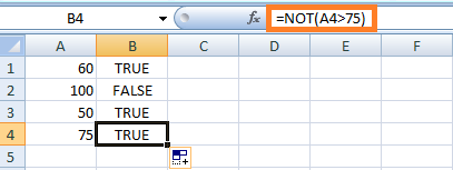

Here in the worksheet, the result will be displayed as TRUE or FALSE, which is the reversed result of the VALUE.

Example 2: Evaluate the given data using the NOT function

To evaluate the data using the NOT condition, the steps to be followed are

Step 1: Enter the data in the worksheet, namely A1:A5

Step 2: Here, the data present in A1:A5 are calculated, equal to Purple.

Step 3: Select a new cell and enter the formula as = NOT (A1="PURPLE"). Press Enter.

Step 4: The result will be displayed as either TRUE or FALSE in the selected cell. To get the result for the remaining cells, drag the formula toward cell A5.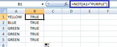

Here in the worksheet, the result will be displayed as TRUE or FALSE as the NOT function reverses the result of the value.

Example 3: Evaluate the given data using NOT and OR function

To evaluate the data using NOT and OR conditions, the steps to be followed are

Step 1: Enter the data in the worksheet, namely A1:A5

Step 2: Here, the data present in A1:A5 are calculated, equal to Purple or Orange.

Step 3: Select a new cell and enter the formula as = NOT (OR (A1="PURPLE", A1="ORANGE")). Press Enter.

Step 4: The result will be displayed as either TRUE or FALSE in the selected cell. To get the result for the remaining cells, drag the formula toward cell A5.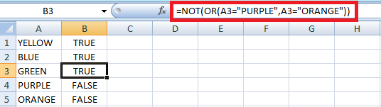

From the above worksheet, the result will be true if any cell range from A1:A5 contains Purple or Orange as the OR function is used. The NOT function reverses the result of the value.

Example 4: Evaluate the given data using NOT and AND function

To evaluate the data using NOT and AND conditions, the steps to be followed are given below:

Step 1: Enter the data in the worksheet, namely A1:A5

Step 2: Here, the data present in A1:A5 are calculated, equal to Purple or Orange.

Step 3: Select a new cell and enter the formula as = NOT (AND (A1="PURPLE", A1="ORANGE")). Press Enter.

Step 4: The result will be displayed as either TRUE or FALSE in the selected cell. To get the result for the remaining cells, drag the formula toward cell A5.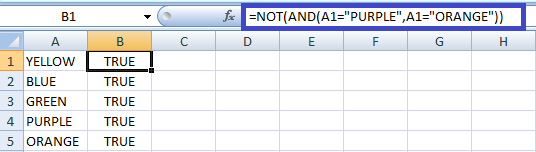

From the above worksheet, the result will be true if all of the cell ranging from A1:A5 contains Purple and Orange as AND function is used. If any of the conditions are evaluated as False, the result will be declared false. The NOT function reverses the result of the value.

Example 5: Evaluate the given data using the NOT function

Here in this example, two cells are evaluated using the NOT function. The steps to be followed are given below:

Step 1: Enter the data in the worksheet, namely A1:A5

Step 2: Here, the data in A1:A5 are calculated to determine whether the value present in A1:A5 is greater than that in B1.

Step 3: Select a new cell and enter the formula as = NOT (A1>B1). Press Enter.

Step 4: The result will be displayed as either TRUE or FALSE in the selected cell. To get the result for the remaining cells, drag the formula toward cell A5.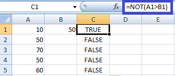

The result in the worksheet will be displayed as TRUE or FALSE. The given argument checks whether the cell range A1:A5 is greater than the value present in cell B1. The NOT function reverses the value of the result.

XOR Function

One logical function is called XOR Function, which performs the exclusive OR function while calculating data. It returns the result as TRUE or FALSE based on the following conditions,

If the given two conditions are true, it returns FALSE.
If given two conditions are false, it returns FALSE
If either of the two conditions is true, the result is TRUE.

Syntax

Parameters

Logical 1- The required logical argument which is evaluated as True or False

Logical 2- It is an optional argument that is evaluated as True or False

Some of the examples of the XOR Function are as follows,

Example 1: Evaluate the given data using the XOR function

Here in this example, two cells are evaluated using the XOR function. The steps to be followed are given below:

Step 1: Enter the data in the worksheet, namely A1:A2

Step 2: Here, the data present in A1:A2 are calculated whether the value present in A1:A2 is greater than 50 and equal to 75

Step 3: Select a new cell and enter the formula as = XOR (A1>50, A1=75). Press Enter.

Step 4: The result will be displayed as either TRUE or FALSE in the selected cell. To get the result for the remaining cells, drag the formula toward cell A2.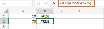

From the worksheet, the logical condition was evaluated as FALSE, FALSE for the value present in cell A1. Hence the result is FALSE. The logical condition for the value present in cell A2 is evaluated to be TRUE, FALSE. Here one of the values is FALSE; hence the result is TRUE.

Example 2: Evaluate the given data using the XOR function

Here in this example, two cells are evaluated using the XOR function. The steps to be followed are given below:

Step 1: Enter the data in the worksheet, namely A1:A2

Step 2: Here the data present in A1:A2, are calculated whether the value present in A1 is equal to "Orange" and A2 >70

Step 3: Select a new cell and enter the formula as

= XOR (A1=ORANGE, A2>70). Press Enter.

Step 4: The result will be displayed as either TRUE or FALSE in the selected cell. To get the result for the remaining cells, drag the formula toward cell A2.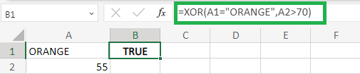

From the worksheet, the logical condition is for the value present in A1 to be evaluated as TRUE and for cell A2 to be evaluated as FALSE. Hence the result will be displayed as TRUE.

Example 3: Evaluate the given data using XOR Function

Step 1: Enter the data in the worksheet, namely A1:E2

Step 2: Here the data present in A1:E2, are calculated using the XOR function based on the values present in it.

Step 3: Select a new cell, F1, and enter the formula as =XOR (A1:E1).Press Enter.

Step 4: The result will be displayed as either TRUE or FALSE in the selected cell. To get the result for the remaining cells, drag the formula toward cell E2.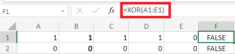

From the worksheet, the result will be displayed as FALSE for the data range A1:E1 and FALSE for the data range A2:F2. The XOR function returns only true if the number of true values is odd. In A1:E1, the number of true values is even; in A2:B2, the number value is zero.

Example 4: Evaluate the given data using XOR and IF function

Here the data is evaluated using XOR and IF functions, and the condition used is true or False.

Step 1: Enter the data in the worksheet, namely A1:E5

Step 2: Here, the data present in A1:E5 are calculated using the XOR function based on its values.

Step 3: Select a new cell namely F2 and enter the formula as = IF (XOR (B 2="Won", C2="Won"), "Yes", "No").Press Enter.

Step 4: The result will be displayed as Yes or No in the selected cell. To get the result for the remaining cells, drag the formula toward cell F5.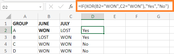

The worksheet evaluates the result as Yes if one of the given values is evaluated as True. The result is evaluated to be No if both the values are evaluated as True or False

Example 5: Evaluate the given data using the XOR function

Here the data is evaluated using the XOR function, and the condition used is greater than

Step 1: Enter the data in the worksheet, namely A1:E5

Step 2: Here, the data present in A1:E5 are calculated using the XOR function based on its values.

Step 3: Select a new cell namely F2 and enter the formula as = XOR (A2>10, B2>15, C2>40, D2>50, E2>70).Press Enter.

Step 4: The result will be displayed as either TRUE or FALSE in the selected cell. To get the result for the remaining cells, drag the formula toward cell F5.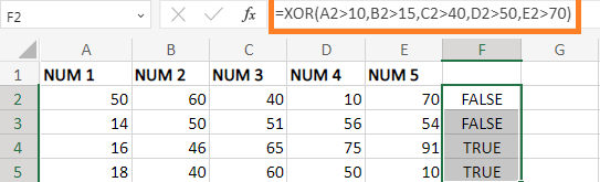

From the worksheet, the result will be displayed as TRUE or FALSE in the cell range F2:F5, where the result TRUE will display if several odd TRUE values are present or else FALSE will display.

Note: The XOR function returns the #VALUE! If there is no logical value present as an argument.

If more than two logical conditions are present as an argument, it returns TRUE if an odd number of True values is present and returns False if not.
The XOR function accepts 1 to 254 conditions as an argument.
Empty references are ignored in the XOR function.
The XOR function evaluates the arguments to TRUE or FALSE, which contains logical arguments.

Summary

The logical functions are used in Excel for calculating the data based on the requirement. From the article, the functions and formulas of logical functions are explained clearly.

Next TopicRegex Formula in Microsoft Excel

← prev next →