How to calculate average in Excel

MS Excel, or Microsoft Excel, is the world's most popular spreadsheet software that enables users to record massive amounts of data and perform various operations. It makes it easier to perform analytical tasks and mathematical calculations on the recorded data in cells across worksheets. Finding an average (also called arithmetic mean) is one commonly used mathematical task we often perform in Excel.

In this tutorial, we discuss various step-by-step methods on how to calculate averages in Excel. Before discussing the different methods of calculating average in Excel, let us first briefly introduce the definition of average and its usage in Excel.

What is Average in Excel?

In Excel, the average is categorized as one of the statistical functions that help us retrieve the arithmetic mean value for a given series of many numeric figures. In particular, the average value is calculated by adding all the given numeric values and then dividing the sum results by the total number count of values we added in the sum calculation. Although it seems easy to calculate the average for a small group of numbers, it becomes difficult and prone to errors when dealing with larger data sets. This is where some programs like Excel come into play.

We can easily calculate the average for massively given numeric values and minimize human errors using an Excel program. There can be many cases when we might need to calculate the average. For instance, we can calculate the average sales of any specific item for the last 12 months in a business.

How to calculate the average in Excel?

Since different averages are based on the given data, Excel offers various methods to calculate the average. Some of the commonly used methods include the following:

Calculating Average in Excel: General Method

Since the average for numbers can be calculated by adding all numbers and dividing their results, we can use the SUM and COUNT functions in Excel to apply this concept.

For example, suppose we have given the following numbers: 15, 10, 30, 20, 25. To calculate the average, we first add all numbers like this: 15+10+30+20+25. Next, we divide the sum by 5 as the total Count of numbers is 5.

Thus, the average, in a mathematical way, is calculated like this:

15+10+30+20+25/ 5

The result for the above calculation is 20, so the average.

If we want to calculate this in Excel, we can use the formula with SUM and COUNT functions like this:

= SUM(15,10,30,20,25)/COUNT(15,10,30,20,25)

Additionally, if the five numbers are recorded in a range A1:A5, we calculate the average and record the result in cell A6 using the below formula:

= SUM(A1:A5)/COUNT(A1:A5)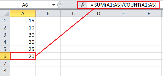

The above image in Excel also shows the same average result as we obtained above mathematically.

Calculating Average in Excel: AVERAGE function

The AVERAGE function is an existing Excel statistical function that is most widely used to calculate the averages (arithmetic mean) in an Excel sheet. The function is mainly helpful when there is no specific limitation when calculating averages. The AVERAGE function can accept up to 255 individual arguments, including numbers, cell references, ranges, arrays, or constants.

Syntax

The syntax of the AVERAGE function in Excel is defined as below:

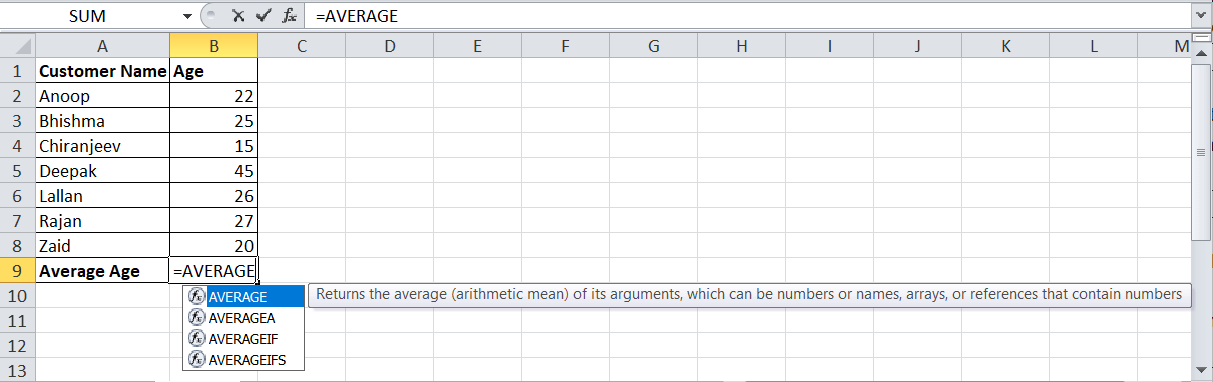
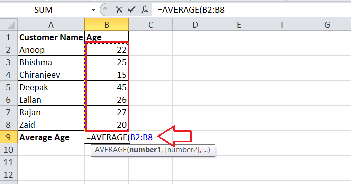
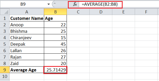
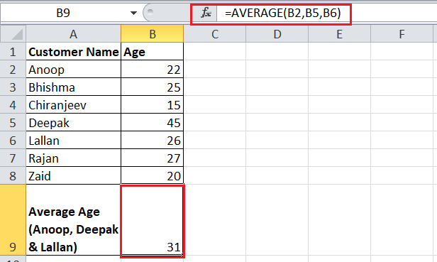
Where number1 is the required argument and number2, number3, and more are additional/ optional arguments for which we need to calculate the average. Although only one argument is mandatory, we are most likely to use at least two arguments to calculate the average.

Steps to use the AVERAGE function

Let us now understand the application of the AVERAGE function with an example. Suppose we have given an Excel sheet with some customers' names in column A (A2:A8) and their respective ages in column B (B2:B8). We need to calculate the average age of all the customers in cell B9.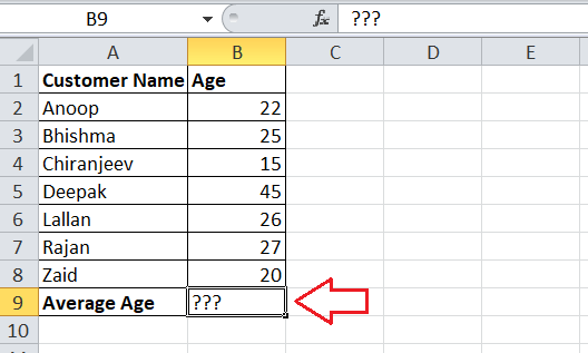

We can perform the below steps to calculate the average age in our example Excel sheet:

• First, we need to select the resultant cell to record the average result. In our example, we select cell B9.
• Next, we need to apply the AVERAGE formula and supply the necessary arguments to it. For this, we first enter the equal (=) sign and then type the function name (i.e., =AVERAGE).
  
• After typing the function name, we must enter the opening parenthesis and pass the individual cell references or a range in the formula. Since we have adjacent cells, we can select or enter the range B2:B8 directly in our formula.
  
• Once the arguments have been given in the formula, we must enter the closing parenthesis and press the ENTER key on the keyboard. This will immediately calculate the average for the given data set. The below image shows the average age of the customers in our example:
  
  Although we used the adjacent cells (or a range) in this example to calculate the average, we can also use the non-contiguous cells as the arguments in the formula. We need to select each desired non-contiguous cell by holding the Ctrl key on the keyboard. After that, we must separate them using the Commas.
  Suppose we want to calculate the average age for three customers, Anoop, Deepak, and Lallan. We can use the AVERAGE function in the following way:
  =AVERAGE(B2,B5,B6)
  
  We can use the AVERAGE function with mixed arguments, empty cells, texts, logical values, and zeros. However, the function ignores the empty cells and values like text and logical values while calculating the average. But, the cells containing zeros are included.

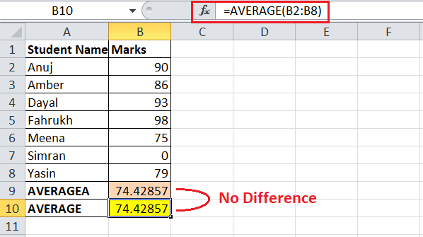
Calculating Average in Excel: AVERAGEA function

The AVERAGEA function in Excel also helps us calculate the average or arithmetic mean of the desired arguments within the worksheet. The function has been available in all the versions of Excel since Excel 2007. The AVERAGEA function is mainly used to eliminate the discrepancy of the AVERAGE function and can include or accept all data types (or values) within a distribution.

Unlike the AVERAGE function, the AVERAGEA function evaluates the text values as zeros. Furthermore, the logical values are also treated differently by the AVERAGEA function. It evaluates the logical value TRUE as 1, while the logical value FALSE is evaluated as 1.

Syntax

The syntax of the AVERAGEA function in Excel is defined as below:

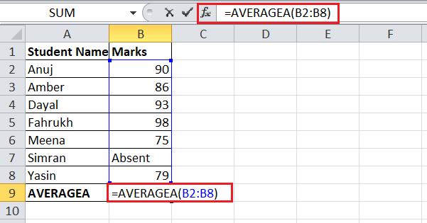
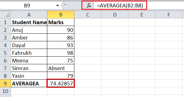
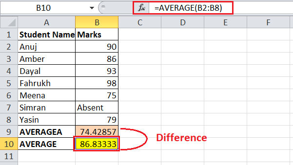
Like the AVERAGE function, the first argument in the AVERAGEA function is mandatory, while other subsequent values are optional. Also, the AVERAGEA function can accept a maximum of up to 255 arguments, which can be numbers, cell references, ranges, arrays, or constants.

Although the syntax and application of both functions, AVERAGE, and AVERAGEA, seem similar, they are different as the AVERAGEA function can calculate the average of given cells with any data like the numbers, text values, and Booleans. In contrast, the AVERAGE function only calculates the given data set's average with numbers.

Steps to use the AVERAGEA function

The application of the AVERAGEA function is precisely the same as the AVERAGE function. Let us now take an example of the following Excel sheet where we have some students' names (range A2:A8) and their marks (range B2:B8). We need to calculate the average of marks using the AVERAGEA function in cell B9.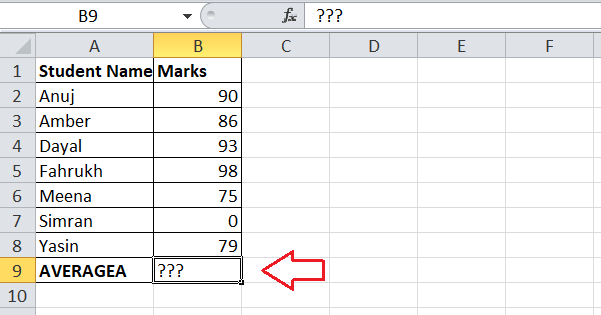

We can apply the AVERAGEA formula by performing the below steps:

• First, we must select the resultant cell B9 to record the average result.
• Next, we must enter the AVERAGEA function followed by the equal sign. We must start the parenthesis, enter/ select the effective range B2:B8, and close the parenthesis.
  
• After clicking the ENTER key, we get the average marks of the students in cell B9, as shown below:
  
  We see a difference between both results if we now calculate the average marks using the AVERAGE function in cell B10. It occurs as the division Count number is different for both functions.
  For the AVERAGEA function, the Count is 7 as the text field is also evaluated as a valid value. But, the division count for the AVERAGE function is 6 as it ignores the text data. So, the difference in results by the functions AVERAGE and AVERAGEA occurs in Excel.
  However, by changing the text value (absent) in cell B7 to zero (0), we get the same result from both functions because both include zero values when calculating the average.
  

Calculating Average in Excel: AVERAGEIF function

The AVERAGEIF function is another existing function that enables users to calculate the average for the given data set. Unlike the AVERAGE and AVERAGEA functions, the AVERAGEIF function also enables users to apply any specific criteria, meaning the average will be calculated for numbers following the applied criteria. With the AVERAGEIF function, Excel first looks in the given data set for a stated criteria/condition. It then calculates the arithmetic mean of the effective resultant cells that follow or satisfy those particular criteria.

Syntax

The syntax of the AVERAGEIF function in Excel is defined as below:

Where the range, criteria, and average range are the arguments of the AVERAGEIF functions.

• Range: It is a mandatory argument used to represent the area/ location on the sheet that contains cells with data required to be tested against the given criteria or condition.
• Criteria: It is another mandatory argument used to specify a rule/ condition to include only the specific cells or data while computing the averages. The criteria we need to specify here may include numbers, text values, logical expressions, cell references, or a range.
• Average_range: It is an optional argument used to specify the range of cells where we want to calculate the average. If average_range is not specified, the function uses the range by default.

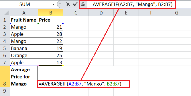
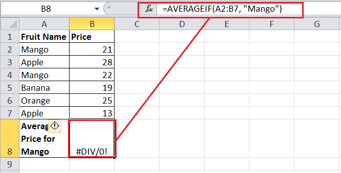
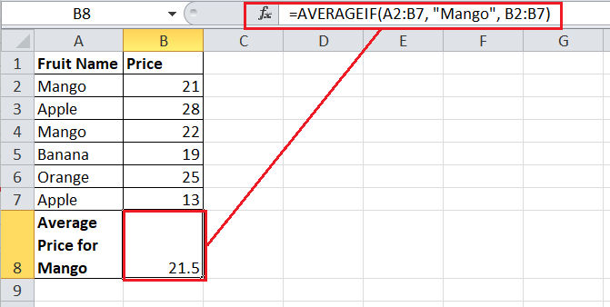
Steps to use the AVERAGEIF function

Let us take an example of the following Excel sheet where we have the names of some fruits (A2:A7) with their prices (B2:B7). Some fruits are also repeated with different prices.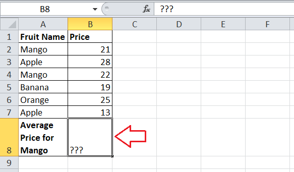

Suppose we only want to calculate the average price for any specific fruit (i.e., Mango) in cell B8. We can use the AVERAGEIF function and calculate the average price for Mango in the following way:

• First, we need to select cell B8 to record the average price for the Mango.
• Next, we enter the AVERAGEIF formula in the following way:
  =AVERAGEIF(A2:B7, "Mango", B2:B7)
  Where A2:B7 represents the range, Mango represents the desired criteria, and B2:B7 represents the average_range.
  
  Although the average_range is optional, we had to specify this to include only the cells with numbers (prices). In our example, if we don't specify the average_range, the function will take the entire range A2:B7 where there are also text values. This will result in #DIV! error.
  
• After entering the formula, we must press the Enter key on the keyboard to retrieve the formula result.
  

Calculating Average in Excel: AVERAGEIFS function

The working concept of the AVERAGEIFS function in Excel is similar to the AVERAGEIF function, although the AVERAGEIFS function allows multiple criteria to be tested while calculating the average. However, the AVERAGEIF function only allows one condition at a time. Unlike the AVERAGEIF function, the AVERAGEIFS function also includes the cells containing TRUE and FALSE, which is somehow required in some cases to test multiple criteria.

Syntax

The syntax of the AVERAGEIFS function in Excel is defined as below:

Where the average_range, criteria1_range2, and criteria1 are the mandatory arguments of the AVERAGEIFS functions. All other arguments are optional and used according to the given data set. Additionally, criteria1 is the rule/condition to be used on the specified range1, while criteria2 is the condition for the range2 and more.

Steps to use the AVERAGEIFS function

Let us take the same example datasheet that we used for the AVERAGEIF function. In that sheet, we have the names of some fruits (A2:A7) with their prices (B2:B7). Some fruits are also repeated with different prices.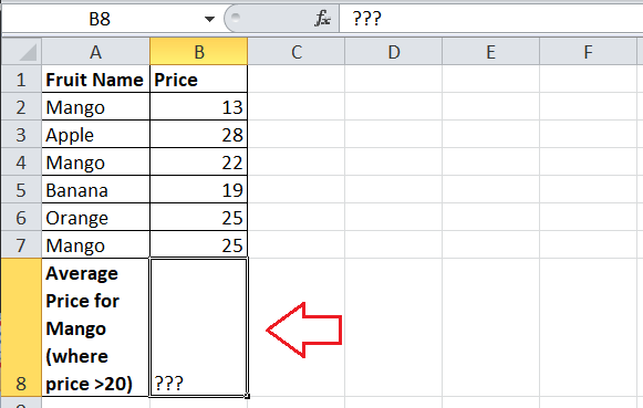

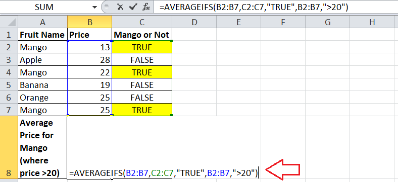
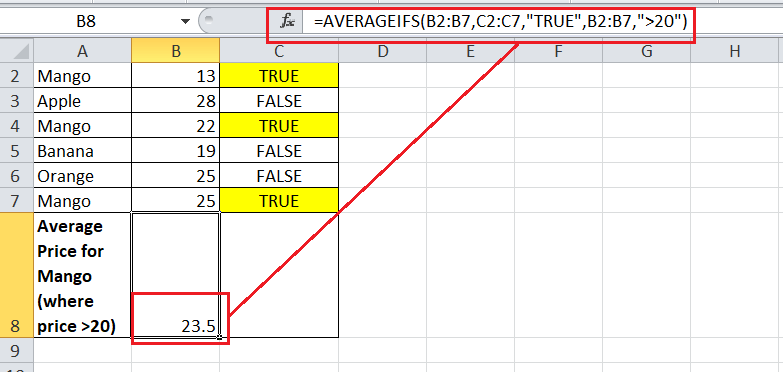
In the previous example, we calculated the average price for the Mango based only on one criteria/ condition. Now, we need to calculate the average price for the Mango that has prices of more than 20. So, we have to use the two criteria:

First: For the range A2:A7, the only condition (criteria) is "Mango", and three rows satisfy this condition

Second: For the range B2:B7, the condition (criteria) is ">20", and only two out of three rows with the Mango satisfy this condition

So, the average prices will be calculated using the following mathematical operation:

(22+25)/2 = 23.5

However, we need to use the OR logical operator to test multiple conditions in Excel. It returns either TRUE or FALSE based on the condition of satisfaction. For instance, if we want to test if the cell A1 contains "Mango" or "Apple", we can use this:

=OR(A1="Mango", A1="Apple")

In our case, we check the condition only for the "Mango" in the entire range A2:A7 in the following way: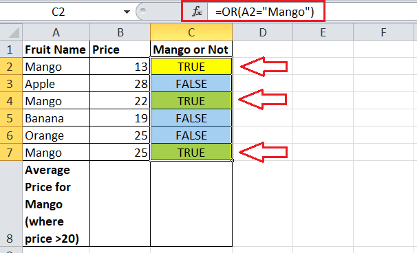

We only apply the OR condition =OR(A2="Mango") in cell C2 and copy it to the remaining cells below.

As displayed in the above image, the OR query result is added in the new column C as TRUE and FALSE. Next, we must use this result and calculate the average by matching only the TRUE values for the range B2:B7.

Since we need to apply multiple criteria while calculating the average, we use the AVERAGEIFS function using the following steps:

• Like applying the other Excel functions, we first need to select the resultant cell to record a result. So, we select cell B8.
• Next, we enter the equal sign, type the function name AVERAGEIFS and enclose the required arguments within the parenthesis signs in the following way:
  =AVERAGEIFS(B2:B7,C2:C7,"TRUE",B2:B7,">20")
  
  Here, we only considered the fruit name "Mango" by following the TRUE results and only those that have prices above 20.
• Lastly, we press the ENTER key on the keyboard, and the average price is returned immediately, i.e., 23.5. It is the same as our mathematically calculated average result.
  

Special Cases

There are many scenarios we may face while computing average results in Excel. However, the following are the two most common scenarios, and we should be cautious while computing the average in such cases.

Calculating Average in Excel Including Zeros

To calculate the average with zero values, we can use the AVERAGE function as usual and pass the cells with zero values in them.

When calculating the average using the Excel AVERAGE function, the formula ignores the text or logical values and the empty cells. However, zero values are included as they are considered valid by the formula. So, the total number count increases, and the overall average of the distribution decreases.

For example, the following sheet has average marks of two different students where student A is absent in one subject while student B has zero (0) marks in one subject.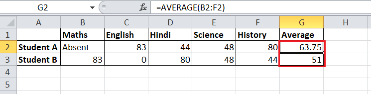

Although marks in total subjects are the same, the average results vary for both students. For student A, the sum of marks is divided by 4. However, for student B, the sum of marks is divided by 5 because a zero value is included here. Therefore, we must explicitly exclude zeros if we don't want to include zero values in our average results.

Calculating Average in Excel Excluding Zeros

We can use the AVERAGEIF function with a little trick to calculate the average, excluding the zero values. Since the AVERAGEIF function enables us to set certain criteria, we can use the below criteria to calculate the average without including the zeros:

=AVERAGEIF(cell or a range,">0")

The above formula will ignore the cells with zero values and the text and logical values.

If we now apply the AVERAGEIF formula in our example data, we get the same average marks for students A and B.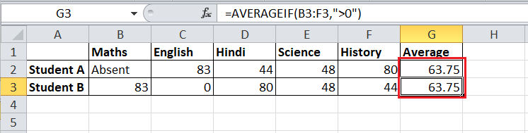

Excel has ignored the zero value cell this time, and so the Count number has decreased from 5 to 4 for student B.

We can also ignore zeros using the AVERAGE function. It is useful when we have a small data set. However, we must carefully use the cell reference or the direct numbers in the formula to eliminate errors. In the same example, we can calculate the average for the student B using the AVERAGE function without involving zeros in the following way:

=AVERAGE(B3,D3,E3,F3)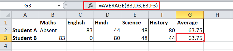

However, it is not usually convenient as we cannot copy-paste the corresponding formula for other resultant cells in this way.

Important Points to Remember

• When using the AVERAGE function to calculate the average in Excel, we must be very cautious. If the supplied arguments are error values or texts that cannot be translated into numbers, the function will lead to unexpected results or errors.
• We can only specify one condition when calculating the average using the AVERAGEIF function.
• The AVERAGEIF function in Excel ignores the empty cells in its argument average_range. If the given range is blank or contains only the text values, the AVERAGEIF function returns the #DIV! error.
• If any cell in the given criteria within the AVERAGEIF function is empty, the function evaluates it as a zero (0) value cell.
• Instead of typing the function name in a resultant cell, we can select the desired function from the Excel Function List. For the average based functions, we can go to Formulas tab > More Functions > Statistical Functions > AVERAGE/ AVERAGEA/ AVERAGEIF/ AVERAGEIFS. This eliminates the human errors of misspelled function names.