| |

Excel LOOKUP() functionExcel offers a function named LOOKUP() function to find an approximation match of data. It performs a rough match lookup either in one-row or one-column range. However, the LOOKUP() function searches for a value itself or its approximate match within a range of column/row. For example, The LOOKUP() function is useful when you don't have the exact value you are looking for. So, we use its nearby value to find the exact result that we want. The LOOKUP() function will help us to search for its exact or nearby match within a range. In MS Excel, this function is categorized under the Lookup and Reference functions inside the formula bar. You can access it from the Formula tab and provide the values to their respective field in its user interface. You can also use it directly in the formula bar by its syntax. Besides this, you can use it many other uses. Need of LOOKUP() functionLet's take a scenario to understand the need for LOOKUP() function in Excel. For example, we have a worksheet containing a list of product id, product name, and price. These columns are containing a lot of data. A user has a requirement to find the product name, whose price is 829 or around it. LOOKUP() function will help us to achieve this result. We will use the LOOKUP() function to find the product name for this value. SyntaxThis function has very different parameter values in which the first two are essential and the third one is optional. On some Excel tutorial websites, you might get one more syntax for the LOOKUP() function. First syntax is given above and another one is - You can consider this syntax same as syntax1 without [result_vertor] parameter. ParametersThe Lookup() function consists of three parameters and all three are important to look for the value and return the result. Lookup_value - The first parameter of this function is lookup_value that holds the value for which the user is searching within the lookup_range. Lookup_range or array - The lookup_range parameter holds the range of cells in which we look for the lookup_value. These range of cells can be either one-row or one-column. [result_vector] (Optional parameter) - The result_vector is the most important but optional parameter of this function. It also consists of a range of cells corresponding to the lookup_range. When the nearby match (approximate match) is found within the lookup_range, the LOOKUP() function picks the adjacent value from result_vector and returns it back to the users. Return valueThe LOOKUP() function returns any type of data depends on the parameter passed in LOOKUP() function. It can be a number or string. Additional result: If the LOOKUP() function is unable to find the exact match for the value (lookup_value) we are searching for, it returns the largest value from the lookup_range that is less than or equal to the value. What is the use of result_vector?As we know that the [result_vector] is an optional parameter, it's your choice that you will use it or not.
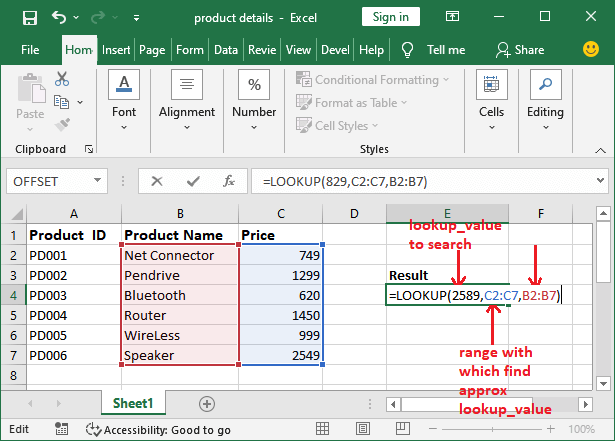
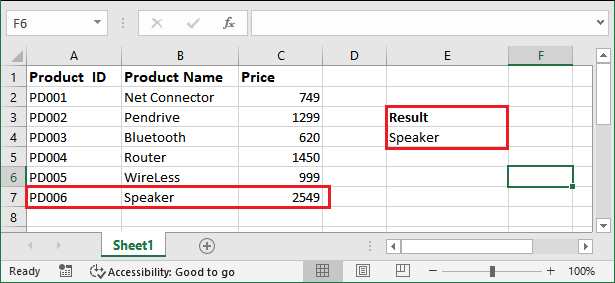
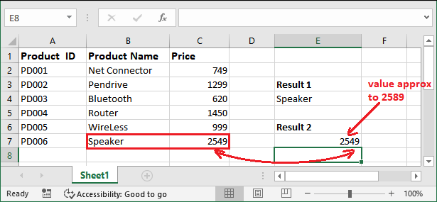
To understand the LOOKUP() function, it is important to learn with example, to know the practical working. We will later understand the usage of this parameter below in this chapter with the help of examples. How to use LOOKUP() function?We have several examples to learn the LOOKUP() function by providing different parameter values. These examples will help you learn it better. We will use both syntaxes to see what values they will return when applying on Excel data. Example 1: With [result_vector] parameterWe have a worksheet containing a list of product id, product name, and price. A user wants to find the product name, whose price is 2589 or around it. We will use LOOKUP() function to find the product name for this value. 
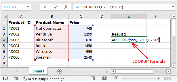
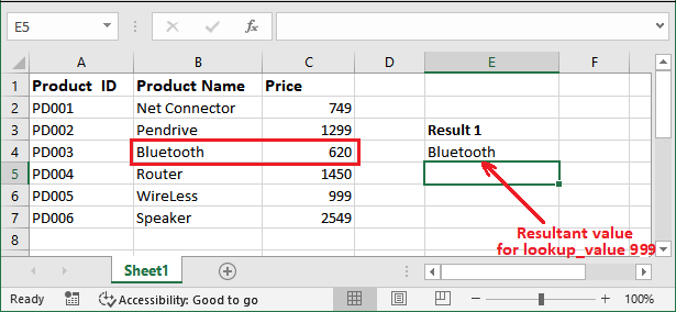
Let's see how we can achieve this result using the LOOKUP() function and how it will help us to achieve this result. Steps to use LOOKUP() function
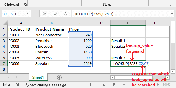
Example 2: Without using [result_vector] parameterIn case we don't use the third parameter inside the LOOKUP() function, it is a big question that what it will return to the user on finding approximate value. We will use the same values used in the above example so that you can compare both results.
Problem with LOOKUP() functionYou may face the problems with LOOKUP() function while using it on Excel data. Sometimes, it does not return the nearest approximate value to the lookup_value. Let's see with an example which type of problem you may face with LOOK() function.
Cause and SolutionThere can be two reasons for returning the incorrect value:
Excel offers a function called VLOOKUP(). You can use it as an alternative to LOOKUP() function. It does not require lookup_range values to be sorted in ascending order. Things to remember while using LOOKUP() functionFollowing are things you should remember while applying the LOOKUP() formula on Excel data.
Hence, you should avoid them while working on Excel data and using the LOOKUP() formula. Verify different resultant valuesBased on this Excel spreadsheet, we will analyze the results for the different lookup_value in LOOKUP() function. 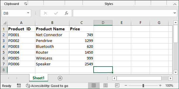
Next TopicMS Excel Grade Formula
|
 For Videos Join Our Youtube Channel: Join Now
Feedback
- Send your Feedback to [email protected]
Help Others, Please Share


