Excel Address Function With Formulas

What is Address Function?

In Excel, the ADDRESS function returns a text string that represents the address of a cell based on its row and column numbers.

Syntax

The syntax of the ADDRESS function is as follows:

Parameters

The function takes three arguments: row_num, column_num, and [abs_num]. Here's a breakdown of each argument:

1. row_num is the row number of the cell you want to reference.
2. column_num is the column number of the cell you want to reference.
3. abs_num (optional) specifies the type of reference: 1 for absolute (with $) and 4 for relative (without $). The default is 1.
4. A1 (optional) is a logical value that specifies the reference style. If a1 is TRUE or omitted, the address is returned in A1-style; if it is FALSE, it is returned in R1C1-style.
5. sheet_text (optional) is the name of the worksheet you want to reference. If sheet_text is omitted, the address is returned for the current sheet.

For example, the formula =ADDRESS (2, 3) returns the text string "$C$2", which is the address of the cell in column C and row 2.

The output of the ADDRESS function is a text string that represents the cell reference based on the input arguments.

Purpose of Address Function

The ADDRESS function in Excel returns a specified cell's cell reference (address) based on the row and column numbers provided as arguments to the function. The function can be used for a variety of purposes, such as:

1. To dynamically create cell references in a formula:

The ADDRESS function can create a cell reference that changes based on the values in other cells or other criteria. For example, you can use the ADDRESS function in a VLOOKUP formula to dynamically reference a different cell based on the value in a dropdown list.

2. To create a text representation of a cell reference:

The ADDRESS function can be used to create a text representation of a cell reference, which can be useful when working with macros or other programming tools.

3. To create a dynamic named range:

The ADDRESS function can be combined with other functions, such as the INDIRECT function, to create a named range that changes dynamically based on the values in other cells.

Overall, the ADDRESS function in Excel is a powerful tool that allows users to create dynamic cell references and text representations of cell addresses, which can help to streamline their workflows and increase their productivity.

Absolute cell reference

An absolute row reference is designated by placing a dollar sign ($) before the row number in a cell reference. For example, $A$1 refers to cell A1 with an absolute row reference. When you copy a formula that contains an absolute row reference, the row number remains the same regardless of where you paste the formula. This is useful when referring to the same row in a range of cells in a formula.

Relative column reference

A relative column reference, on the other hand, is designated by not using a dollar sign ($) before the column letter in a cell reference. For example, A1 refers to cell A1 with a relative column reference. When you copy a formula that contains a relative column reference, the column letter is adjusted based on where you paste the formula. This is useful when referring to different columns in a range of cells in a formula.

Arguments used in Address Function

1 (default): Returns a relative reference (e.g., A1)

2: Returns an absolute reference with the row number fixed (e.g., $A1)

3: Returns an absolute reference with the column number fixed (e.g., A$1)

4: Returns an absolute reference with both the row and column numbers fixed (e.g., $A$1)

a1 (optional): This parameter specifies the reference style you want to use. It uses the A1 reference style (e.g., A1, B1, C1, etc.) if set to TRUE or omitted. If set to FALSE, it uses the R1C1 reference style (e.g., R1C1, R1C2, R1C3, etc.).

Here's an example of how the ADDRESS function is used:

=ADDRESS (2, 3, 4)

This formula would return the text string "$C$2" because it's the cell reference of row 2 and column 3, with the row and column numbers fixed.

How to use the Address function in Excel?

Using the ADDRESS function, the user can retrieve the possible outcome of the data. The steps to be followed are,

Example 1: Retrieve the address of the cell using Address Function

Step 1: Enter the data in the worksheet as follows,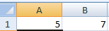

Step 2: In cell C1 enter the formula as = ADDRESS (A1, B1).

Step 3: Press Enter. The ADDRESS function returns the value as $G$5.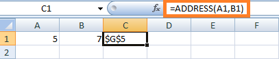

In the formula, the value present in A1 and B1 indicates the 5th row and 7th column, which returns the text string "$G$5", which is the address of the cell in column G and row 5. It is expressed in absolute reference.

Example 2: Create an absolute row and relative column for the given example

To create an absolute row and relative column in the given data, the steps to be followed are,

Step 1: Select a new cell and enter the formula as =ADDRESS (2, 3, 2)

Step 2: Press Enter. The ADDRESS function displays the cell value as a whole row and relative column.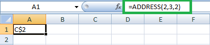

Relative column using reference style

When using relative references in Excel, the reference style adjusts automatically based on the position of the cell that contains the formula.

Example 3: Display the relative column using reference style.

Step 1: Select a new cell and enter the formula as =ADDRESS (2, 3, 2, FALSE)

Step 2: Press Enter. The ADDRESS function displays the relative column in reference style.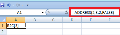

Absolute reference to another workbook and worksheet

To create an absolute reference to another workbook and worksheet, you need to use the following syntax:

='[WorkbookName.xlsx] WorksheetName'! CellReference

where

WorkbookName.xlsx is the name of the workbook you want to reference. If the workbook is in a different folder, you must include the full path to the file.

Worksheet Name is the worksheet's name within the workbook you want to reference.

Cell Reference is the cell you want to reference in the other worksheet.

For example, if you want to reference cell A1 in Sheet1 of a workbook named "Data.xlsx," located in the same folder as your current workbook, you would use the following formula:

= ' [Data.xlsx] Sheet1'! A1

Note: Single quotes are required around the file name and worksheet name, and there is no space between the first single quote and the opening bracket.

Also, make sure that the workbook you are referencing is open. Otherwise, Excel will not be able to retrieve the data.

Example: Create an absolute reference for another worksheet and workbook

Step 1: Select a new cell and enter the formula as =ADDRESS (2, 3, 1, FALSE," [Book 1] Sheet 1").

Step 2: Press Enter. The ADDRESS function displays the result as follows,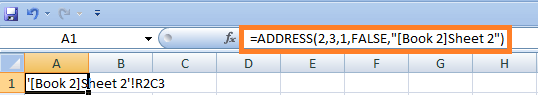

Absolute reference to another worksheet

An absolute reference to another worksheet in Excel requires using the worksheet name and cell reference. Here's the syntax:

'Worksheet Name'! Cell Reference

For example, if you want to refer to cell A1 on a worksheet named "Sheet2" from a formula in cell B1 on the current worksheet, you would use the following absolute reference:

='Sheet2'! A1

Note: The worksheet name must be enclosed in single quotes containing spaces or special characters. Also, the exclamation point (!) is used to separate the worksheet name from the cell reference.

Example: Create an absolute reference to another worksheet

Step 1: Select a new cell and enter the formula as =ADDRESS (2, 3, 1, FALSE, "EXCEL SHEET")

Step 2: Press Enter. The ADDRESS function displays the result as follows,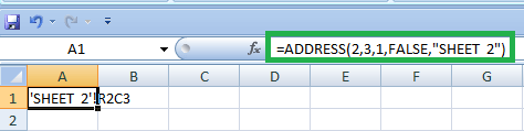

In the formula, Sheet name two is used. Based on the requirement, the Sheet name in the formula is modified.

Relative reference to another Sheet

In Microsoft Excel, a relative reference to another sheet is a formula that refers to a cell or range of cells in a different sheet relative to the current sheet. To create a relative reference to another sheet in Excel, follow these steps:

Step 1: Type an equal sign (=) in the cell where you want to create the formula.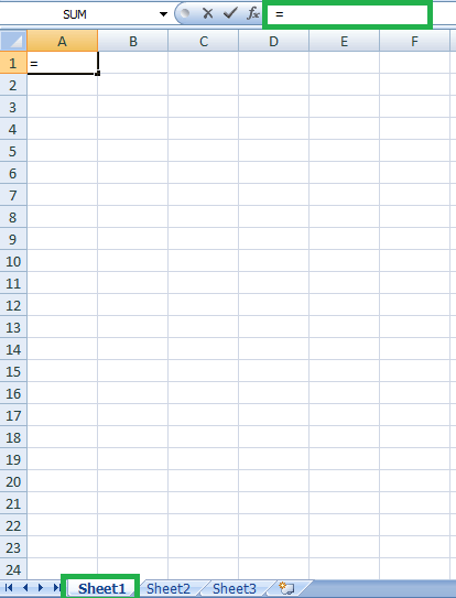

Step 2: Navigate to the other sheet by clicking on its tab at the bottom of the Excel window.

Step 3: Select the cell or range you want to reference.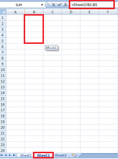

Step 4: Type the cell or range address into the formula, preceded by the sheet name and an exclamation point. For example, if you want to reference cell A1 on a sheet named "Sheet2", you would type "Sheet2! A1" into the formula.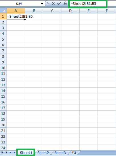

When you copy and paste a formula that includes a relative reference to another sheet, the reference will adjust automatically to the new location based on the relative position of the sheets involved.

How to retrieve the specified cell value by using the Excel address function?

To retrieve a cell value using the Excel ADDRESS function, you can use the following formula:

=INDIRECT (ADDRESS (row_num, col_num))

Here, row_num is the row number of the cell you want to retrieve, and col_num is the column number of the cell you want to retrieve. The ADDRESS function returns the cell address as text, and the INDIRECT function converts the text into a cell reference, which can then retrieve the cell value.

For example, if you want to retrieve the value of cell D1, you can use the following formula:

=INDIRECT (ADDRESS (1, 4))

Here, the row number is 1 (since the cell is in the first row), and the column number is 4 (since the cell is in the fourth column).

The ADDRESS function can also accept a cell reference instead of row and column numbers as its argument. For example, you can use the following formula to retrieve the value of cell D1 by referencing the cell directly:

=INDIRECT (ADDRESS (ROW (D1), COLUMN (D1)))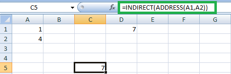

Here, the ADDRESS function returns the address of cell D1, and the ROW and COLUMN functions extract the row and column numbers from the cell reference. The INDIRECT function then converts the address into a cell reference, which can be used to retrieve the cell value.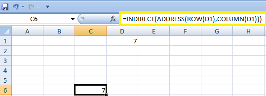

Address of a cell with the Highest Value

To get the address of a cell with the highest value in a range of cells, you can use the following formula:

=ADDRESS (MATCH (MAX (range), range, 0), COLUMN (range))

Here, range refers to the range of cells you want to search for the highest value. The MAX function returns the highest value in the range, and the MATCH function finds the position of that value within the range. The ADDRESS function returns the cell's address with the highest value based on its row and column position.

For example, let's say you have a range of cells A1:A10 and want to find the cell address with the highest value in that range. You can use the following formula:

=ADDRESS (MATCH (MAX (A1:A10), A1:A10, 0), COLUMN (A1))

This will return the cell address with the highest value in the range A1:A10.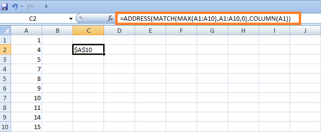

Note: If multiple cells have the same highest value, this formula will return the address of the first cell in the range with that value. Suppose you want to find the address of the last cell with the highest value. In that case, you can use the MAXIFS function (available in newer versions of Excel) to find the maximum value and its position and then use the INDEX function to get the address of the last cell with that value.

How to find the column letter from the column Number?

To find the column letter from the column number using the ADDRESS function in Excel, you can use the following formula:

=ADDRESS (1, column_number, 4)

Here, column_number is the column number you want to find the corresponding letter. The third argument of the ADDRESS function (which is set to 4 in this example) specifies the output format of the cell reference. A value of 4 returns a reference as a column letter and row number.

For example, if you want to find the column letter for column number 10, you can use the following formula:

=ADDRESS (1, 10, 4)

This will return the text string "J1", representing the cell reference for the first cell in column 10.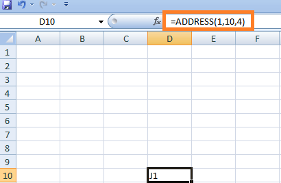

Note: The formula assumes that the column number is between 1 and 16384, the maximum number of columns in Excel. If you need to find the column letter for a column number greater than 16384, you must modify the formula accordingly.

Summary

In conclusion, the ADDRESS function in Excel is a powerful tool for working with cell references. It allows you to dynamically generate cell references based on row and column numbers and provides control over the format of the resulting reference. The function is especially useful when used with other functions, such as INDIRECT, INDEX, and MATCH, to create complex dynamic formulas that reference cells. By understanding how to use the ADDRESS function, you can save time and increase the efficiency of your Excel workflows.