| |

Excel ISERROR() functionAs the name specifies, ISERROR() is a logical function of Excel. It is a special function of Excel that is used to identify whether a cell is going to be referred an error or not. This function is able to detect all types of errors. The ISERROR() function returns TRUE if it found any type of error for that specified cell. Alternatively, if the cell being referred has no error, it returns FALSE as a result. Thus, the cell reference is passed as an argument in this function. This function works on errors - Errors that are generated by Excel on using incorrect value or data, such as - #N/A, #VALUE!, #NUM!, #REF!, #DIV/0!, #NAME?, or NULL. Properties of ISERROR() function
Why use ISERROR() function?There might be a possibility of occurrence of missing value in your Excel data. If the further operation is performed on such data, it will give you an error instead of a valuable result. For example, if you divide a number by 0, it will generate an error, i.e., #DIV/0!. If further operation will be carried out on it, you will get more errors. Thus, before doing such operations, check if there is any error in operations. ISERROR() function is a function that helps you identify the errors that can be occurred due to such operations. Then you can avoid doing these operations, which generate errors. SyntaxThe ISERROR() function takes only one argument, which is mandatory to provide in it.
ISERROR(value)
This value parameter can be a cell reference, a numeric expression, a value, number, or expression to be tested for error. Return valueThe ISERROR() function returns a Boolean value, either TRUE or FALSE (one at a time). It will return TRUE if it finds an error in the given expression. Otherwise, it will return FALSE for not finding any error in the value/expression. ExamplesThere is a list of rough examples using which you can try to learn this for different values.
Now, let us implement these expressions or values with ISERROR() function in an Excel worksheet. Show you all these examples on Excel data so that you can also verify its results. Example 1Step 1: We have the following values and expressions stored in an Excel worksheet. We will check that whether these values or expressions are an error or not. 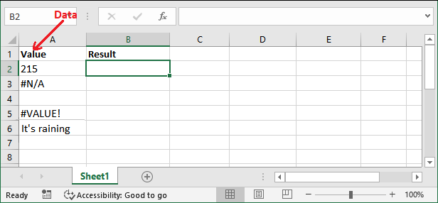
Step 2: Firstly, for A2 cell value, write the following IFERROR() function. =ISERROR(A2) 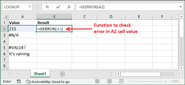
Step 3: Press the Enter key and get the result as a Boolean value, either TRUE or FALSE depending on the expression/value. See that it has returned FALSE for the following expression as it is not an error. 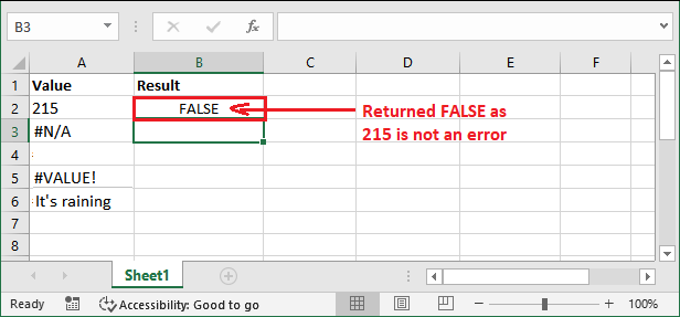
Step 4: Now, we will check the error for another value (cell A3). So, write the following IFERROR() formula for it. =IFERROR(A3) 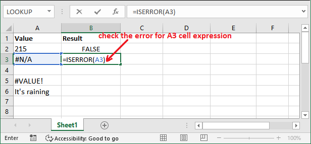
Step 5: Get the result by hitting the Enter key and see what it will return. You can see that it has returned FALSE as this expression contains an error. 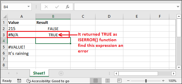
Step 6: See the result for all the expressions, even for a string parameter. 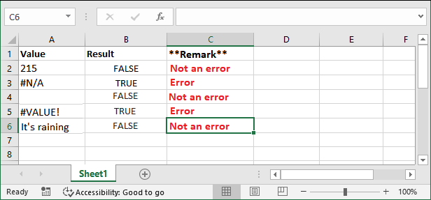
These all above are simple examples for the simple expressions and values, including string parameters. Note: Excel always returns TRUE when it found Excel errors in the expression that is going to be provided inside ISERROR() function.Example 2We will show you an expression. Don't be confused between them. The way of passing the inside ISERROR() function can change the resultant value. We have told you that an expression like 17/0 will generate Divide by 0 error. Let's see an example for it- Step 1: We have a numerical expression (divide by zero) stored in a single B3 cell for which we want to check whether it is an error or not. 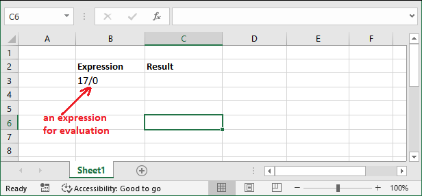
Step 2: Write the IFERROR() formula for it in its adjacent cell. =ISERROR(B3) 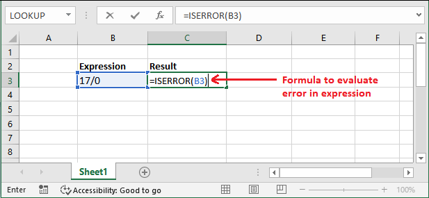
Step 3: Get the result for it by hitting the Enter key. According to our research, it must return TRUE as this expression is an error that generates #DIV/0! Error. But it has returned FALSE. 
It means - this function has taken the A4 cell values (expression - 17/0) as a string and has not found any error. That is why it returned FALSE here. Step 4: To avoid this error, provide these values in different cells like this and then apply the ISERROR() function. 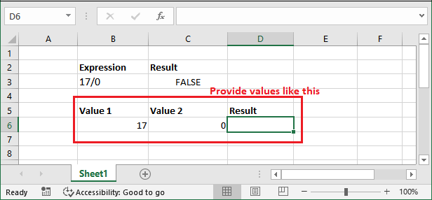
Step 5: For this, write the ISERROR() formula in this way to evaluate the divide by 0 expression. =ISERROR(B6/C6) 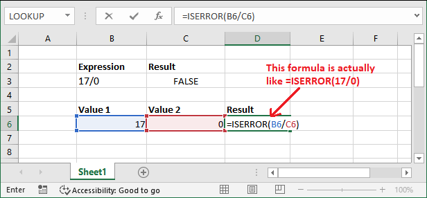
Step 6: Once again, click the Enter key and get the result for it as well. You will now see that it has returned TRUE this time. It means -it has evaluated this expression as an error this time. 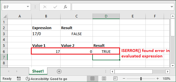
You can compare both results given here and avoid mistakes while providing value inside the function. It was important to learn this example. Note: You might do such common mistakes while evaluating the expressions correctly. So, be careful while using them.Example 3: Count number of errorsIf you wish to count the total number of errors present in an Excel worksheet, you can easily do it with the help of the ISERROR() function. ISERROR() is used with the SUMPRODUCT() function to count the number of errors. This example will show how you can do it: Step 1: See the following data that is containing some normal data and some errors. For this worksheet, we will check the total errors. 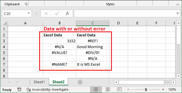
Step 2: Write the following formula using SUMPRODUCT() and ISERROR() for a range of cells (B3:C7). =SUMPRODUCT(--ISERROR( B3:C7)) 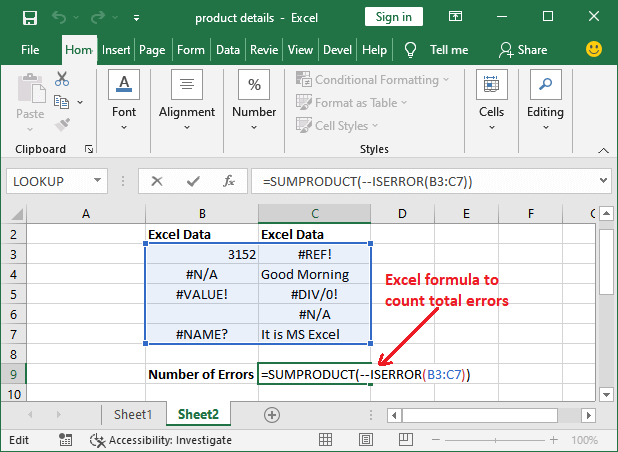
Step 3: To get the count of errors, press the Enter key of your keyboard and see the result. 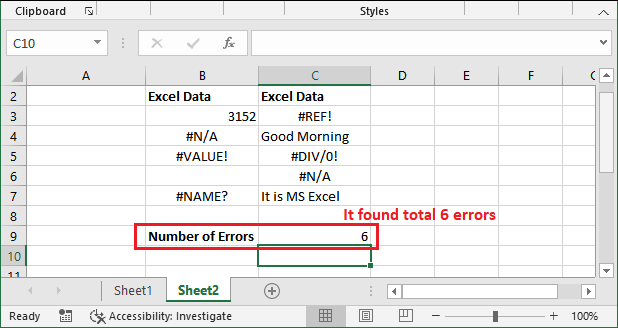
In the same way, you can find and get the sum of total errors for the selected and or in the entire worksheet. How errors are counting using above formula?=SUMPRODUCT(--ISERROR( B3:C7)) The SUMPRODUCT() has accepted one or more arrays and calculated the sum of products for the corresponding numbers. See how all this complete formula worked:
Instead of using SUMPRODUCT() function, you can also use SUM() but you have to press Shift+Ctrl+Enter instead of simply pressing Enter key to get the result. Example 4: Handle ErrorsISERROR() function is used with IF() function to find and handle the error. You can provide a custom message to tell the users regarding error when using the ISERROR() function inside the IF() function. =IF(ISERROR(value),"Custom Error message", value)) Return value If the function found an error, it will return the custom message you have provided. Otherwise, it will return the value itself not finding any error. Steps for custom error message See the following steps how it will actually be done: Step 1: See the given data in which one is an error and another is normal data. Write the following formula firstly for A2 cell. =IF(ISERROR(A2), "It's an ERROR", A2) 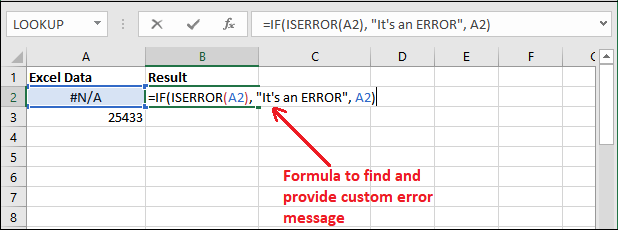
Step 2: Get the result and see that it has returned the custom message "It's an ERROR" as it found a #N/A error. 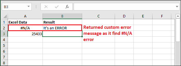
Step 3: Write the formula for the next cell A3 that is containing a numeric number. =IF(ISERROR(A3), "It's an ERROR", A3) 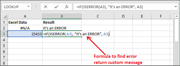
Step 4: This time, it has returned the value itself as it does not find any error in the A3 cell. 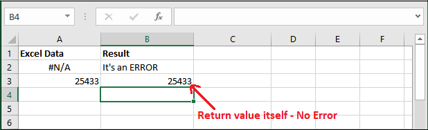
Next TopicExcel add-ins
|
 For Videos Join Our Youtube Channel: Join Now
Feedback
- Send your Feedback to [email protected]
Help Others, Please Share


