Excel Sumif function

Sumif Function

Excel is widely used by many organizations and companies for multipurpose usage. By default it contains multiple functions and formulas which help the user to perform the calculations quickly based on the criteria. Among the various function, one of the familiar function is called Sumif function. Sumif function is used to sum the values in the given range. Based on the requirement the Sumif formula is modified. Criteria like date, text and numbers are applicable to Sumif function. Apart from this the logical operator are wildcards are also used as criteria for partial matching.

Syntax

The syntax for the Sumif function is as follows,

Range - Criteria are applied to range

Criteria - Criteria to apply

sum_range - It is an optional. If sum_range is not present in formula the cell in range are summed.

Some of the examples of the SUMIF function are as follows,

Example 1: How to sum the cells whose value are greater than 50?

To sum the cells value greater than 50, the steps to be followed are,

Step 1: Enter the data in the worksheet namely A1:A5

Step 2: Here to sum the values which are greater than 50, apply the logical operator greater than (>). Select a new cell namely B1 and enter the formula as =SUMIF (A1:A5,">50"). A1:A5 is called range and ">50" is called criteria.

Step 3: Press Enter. The result will be displayed in the cell B1 which is the sum of value greater than 50.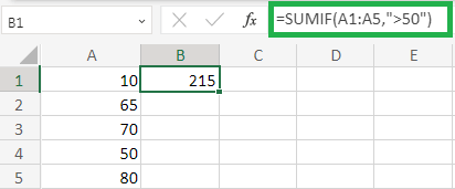

From the above worksheet the result is displayed as 215 which is the sum of (65+70+80) cell values greater than 50.

Example 2: How to sum the cells whose value is equal to 100?

To sum the cells value which is equal to 100, the steps to be followed are,

Step 1: Enter the data in the worksheet namely A1:A5

Step 2: Here to sum the values which is equal to 100, apply the logical operator equal to (=). Select a new cell namely B1 and enter the formula as =SUMIF (A1:A5,"=100"). A1:A5 is called range and "=100" is called criteria.

Step 3: Press Enter. The result will be displayed in the cell B1 which is the sum of value equal to 100.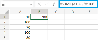

From the above worksheet the result is displayed as 200 which is the sum of (100+100) cell values equal to 100.

Example 3: How to sum the cells whose value is less than or equal to 100?

To sum the cells value which is less than or equal to 100, the steps to be followed are,

Step 1: Enter the data in the worksheet namely A1:A5

Step 2: Here to sum the values which is less than or equal to 100, apply the logical operator less than or equal to (<=). Select a new cell namely B1 and enter the formula as =SUMIF (A1:A5,"<=100"). A1:A5 is called range and "=100" is called criteria.

Step 3: Press Enter. The result will be displayed in the cell B1 which is the sum of value less than or equal to 100.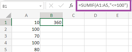

From the above worksheet the result is displayed as 360 which is the sum of (10+100+70+100+80) cell values lesser than or equal to 100.

Example 4: How to sum the cells whose value is not equal to 50?

To sum the cells value which not equal to 50, the steps to be followed are,

Step 1: Enter the data in the worksheet namely A1:A5

Step 2: Here to sum the values which not equal to 50, apply the logical operator not equal to (<>). Select a new cell namely B1 and enter the formula as =SUMIF (A1:A5,"<>50"). A1:A5 is called range and "<>50" is called criteria.

Step 3: Press Enter. The result will be displayed in the cell B1 which is the sum of value not equal to 50.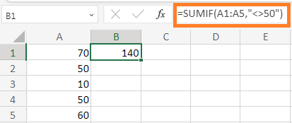

From the above worksheet the result is displayed as 140 which is the sum of (70+10+60) cell values not equal to 50.

Example 5: How to compare single cell with multiple cell using Sumif Function?

To compare single cell with multiple cell, the steps to be followed are,

Step 1: Enter the data in the worksheet namely A1:A5

Step 2: Here to compare the values present in cell A1 with other Cell, select a new cell namely B1 and enter the formula as = SUMIF (A1:A5,">"&A1)

Step 3: Press Enter. The result will be displayed in the cell B1 which is the sum of value greater than the value present in A1. Here concatenation concept is used.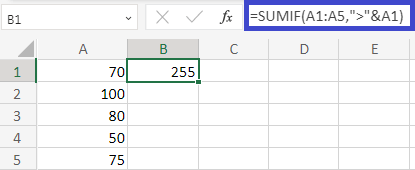

From the above worksheet the result will be displayed as 255 which is the sum of value (100+80+75) greater than value present in cell A1.

Example 6: Sum the cells which are not blank from the given data using Sumif Function?

To count the cells which contains data the steps to be followed are,

Step 1: Enter the data in the worksheet namely A1:A5

Step 2: Here to sum the values in the cell which is not blank, apply the logical operator not equal to (<>). Select a new cell namely B1 and enter the formula as =SUMIF (A1:A5,"<>"). A1:A5 is called range and "<>" is called criteria.

Step 3: Press Enter. The result will be displayed in the cell B1 which is the sum of data present in cell.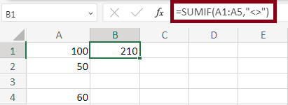

From the above worksheet the result will be displayed as 210 which is the count of value of the cells that containing data which are non-blank.

Example 7: Display the sum value which is equal to any selective color?

Here to display the sum of values which is present equal to any selective color, the respective two columns are compared in the formula. The steps to be followed are,

Step 1: Enter the numeric value and color name in cell A1:A5 and B1:B5.

Step 2: Select a new cell namely C1 and enter the formula as =SUMIF (B1:B5,"blue", A1:A5).

Step 3: Press Enter. The result will be displayed in cell C1 which is the count of values present in cell equal to blue color.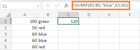

From the above worksheet the result will be displayed as 120 which is the count of values equal to color blue.

Example 7.1 Display the sum value which is not equal to any selective color?

Here to display the sum of values which is not equal to any selective color, the respective two columns are compared in the formula. The steps to be followed are,

Step 1: Enter the numeric value and color name in cell A1:A5 and B1:B5.

Step 2: Select a new cell namely C1 and enter the formula as =SUMIF (B1:B5,"<>peach", A1:A5).

Step 3: Press Enter. The result will be displayed in cell C1 which is the count of values present in cell not equal to peach color.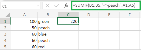

From the above worksheet the result will be displayed as 220 which is count of values present in cell namely A1, A3 and A5.

Example 7.2 Display the sum value which is starting with specified alphabet?

To sum the value starting with specified alphabet, the steps to be followed are,

Step 1: Enter the numeric value and alphabet in cell A1:A5 and B1:B5.

Step 2: Select a new cell namely C1 and enter the formula as =SUMIF (B1:B5,"A*", A1:A5).

Step 3: Press Enter. The result will be displayed in cell C1 which is the count of values present in cell starting with Alphabet A.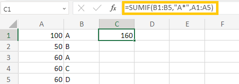

From the above worksheet the result will be displayed as 160 which is the count of values starting with alphabet 'A'.

Example 8: Calculate the blank and non-blank cells in the given data.

To calculate the blank and non-blank cell in the given data, the steps to be followed are,

Step 1: Enter the data in the worksheet namely A6:C6

Step 2: To calculate the blank cells enter the formula as =SUMIF (C2:C6,"", B 2:B6) and to calculate the non-blank cells enter the formula as =SUMIF (C 2:C6,"<>", B2:B6)

Step 3: Press Enter. The sum of blank and non-blank cells will display in the selected cell.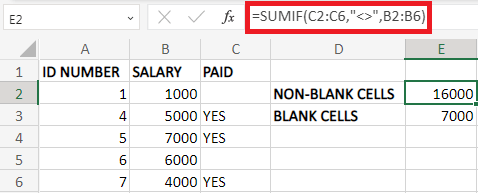

From the given data the sum of blank and non-blank cells are displayed separately using formula.

Example 9: How to compare the date in the cells?

To compare the dates in the cell, the steps to be followed are,

Step 1: Enter the data in respective cell namely A1:B6.

Step 2: Select a new cell namely C1 and enter the formula as =SUMIF (A2:A6,"<"&TODAY (), B2:B6)

Step 3: Press Enter. It calculates the sum of values where the data present in cell is lesser than today's date.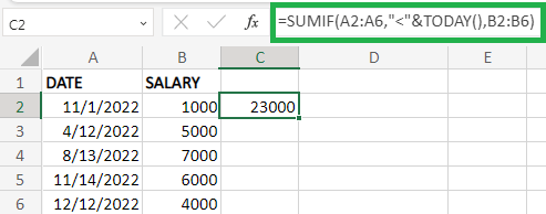

From the above worksheet the result will be displayed as 23000 which is the sum of values lesser than today's date.

Example 10: How to calculate the sum of values for the specified date?

To calculate the Sum of values for the specified date, the steps to be followed are,

Step 1: Enter the data in the worksheet namely A1:B6.

Step 2: Select a new cell and enter the formula as =SUMIF (A2:A6,"<"&DATE (2022, 12, 6), B2:B6).

Step 3: Press Enter. The result will be displayed in the cell which is the sum of values lesser than specified date.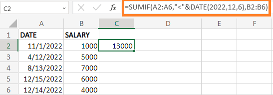

From the above worksheet the result will be displayed as 13000 which is the count of values lesser than specified date.

Example 11: Display the sum of values of color in the given data using not equal to operator?

To display the sum of value of the various color present in the data using not equal to operator, the steps to be followed are,

Step 1: Enter the data in the required column namely A1:B5.

Step 2: Select a new cell and enter the formula as =SUMIF (A1:A5,"<>color name", B1:B5). Similarly the formula is modified for the selected color.

Step 3: The result will be displayed in the respective cell.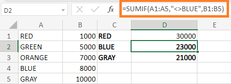

From the above worksheet the sum of values of various color is displayed using not equal to operator.

What are wildcard characters?

As previously explained the wildcard characters are used for incomplete matches. Using wildcards in Excel displays the result which shares the similar pattern. An important characteristic of wildcard is that, it works with text and not with numbers. The wildcard characters are as follows,

? (Question Mark)

*(Asterisk)

~ (Tilde)

The wildcard characters are termed as special characters which replaces the character in the formula.

Some of the examples of Sumif function using Wildcard characters are explained as follows,

Example 1: Display the sum of value of specified count of characters in the given data using wildcard characters?

To display the sum of specified count of characters in the given data, the wildcard character question mark (?) is used. A single question mark matches with one character. The steps to be followed are,

Step 1: Enter the required data in the column A1:B5.

Step 2: Select a new cell and enter the formula as =SUMIF (A1:A5,"?????" B1:B5). Here 5 characters are counted in the data.

Step 3: Press Enter. The result will be displayed in the selected cell which is the sum of value of specified count of characters.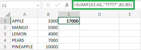

From the above worksheet the result will be displayed as 17000 which is the count of values 5 characters in the data. Similarly the formula can be modified based on the specified count of characters.

Example 2: Display the sum of values starting with specified characters?

To display the sum of values starting with specified characters, the wildcard character Asterisk (*) is used. Asterisk matches any sequence of charactes.The steps to be followed are,

Step 1: Enter the data in the required column A1:A5.

Step 2: Select a new cell and enter the formula as =SUMIF (A1:A5,"AB*", B1:B5). Here Asterisk is placed after the character to count the values of the data starting with AB.

Step 3: Press Enter. The sum of values is displayed in the cell starting with character 'AB'.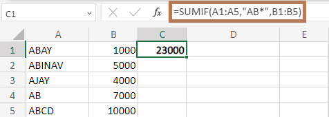

From the above worksheet the result will be displayed as 23000 which is the sum of values starting with character 'AB'.

Example 2.1 What will be the result if the asterisk is not mentioned in formula in the Example 2?

If the wildcard character called Asterisk (*) is not present in the data, the result will be displayed as shown below,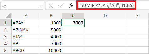

In the above worksheet the formula takes the data which contains only 'AB' as asterisk (*) is not present in the formula. Hence the result will be displayed as 7000.

Example 3: Display the sum of values ending with specified characters?

To display the sum of values ending with specified characters, the wildcard character Asterisk (*) is used. The steps to be followed are,

Step 1: Enter the data in the required column A1:A5.

Step 2: Select a new cell and enter the formula as =SUMIF (A1:A5,"*ES", B1:B5). Here Asterisk is placed before the character to count the values of the data ends with 'ES'.

Step 3: Press Enter. The sum of values is displayed in the cell ends with character 'ES'.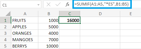

From the above worksheet the result will be displayed as 16000 which is the sum of values ending with character 'ES'. Similarly the formula is modified to find the sum of values for the selective characters.

Summary

From the above tutorial, the various functions and methods to sum the selected value using SUMIF function is explained clearly. Basically SUMIF supports one condition. If the user wants to apply multiple criteria, SUMIFS Function is used.