How to Filter in Excel: add, apply, use, and remove filter

The advancement of Microsoft Excel in today s world is because of its features that allow one to arrange, manipulate and display data in a user-friendly manner. One such Excel feature is the AutoFilter.

The advantage of Excel is that it enables the user to filter any data and offers different built-in options to ease the entire process. This tutorial will cover the various steps to add, apply, use and remove the filter from the Excel worksheet.

1. What is Filter in Microsoft Excel?
2. How to apply filter
3. Steps to add filter to one or multiple columns
4. How to filter empty or non-empty cells
5. How to add Filter for different data values:
   • Filter Text data
   • Filter numeric data
6. Step to apply Filter by color
7. Filter data using search field
8. How to copy the filtered data
9. Re-apply the Filter
10. How to remove the applied filter
11. How to clear the filter
12. Excel filter not working

Let's get started!

What is filter in Microsoft Excel?

Excel Filter (also known as AutoFilter) is a valuable method widely used to show only the relevant data, removing all other information from the worksheet. Using this technique, you can quickly filter rows based on different values, formats, and other customised criteria. Once the filter is applied to your worksheet, you easily copy, edit, insert a chart or print the visible data without rearranging the complete data.

Methods to add filter in Microsoft Excel

In Excel, there are three methods to apply the filter technique:

Method 1: Using Filter button

Go the Data tab, click on Filter option present under Sort & Filter group.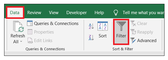

Method 2: Using Filter under Editing group

Click on the Excel Home tab, from the Editing group, go to the Sort & Filter option, click on Filter.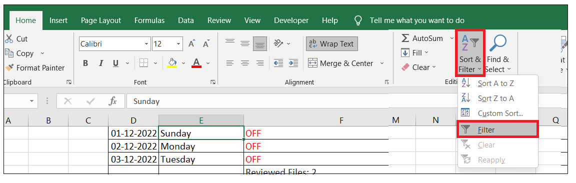

Method 3: Using Excel Filter shortcut

The third method to apply filter in Excel is by using Excel shortcut.

You can easily turn on or off the filter by shortcut: Ctrl+Shift+L

Respective of the method you choose, the following drop-down will appear in the header cells of your Excel worksheet.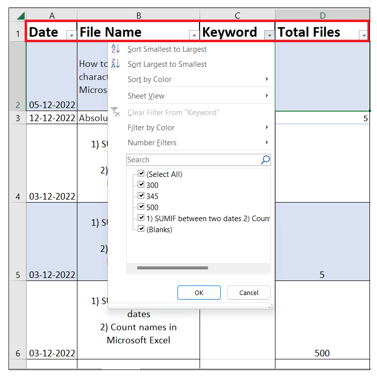

How to apply filter in Excel

In the above section, we covered how to add Filter in an Excel worksheet. Once we add the Filter, a drop-down arrow will be added in the respective column heading. This arrow indicates that the Filter has been added but has yet to be applied when you hover over the arrow, a screen tip displays (Showing All).

Perform the following steps, do filter your Excel data:

1. Move your cursor to the drop-down arrow for the column you want to filter.
2. All the fields of the filter are selected by default, uncheck the Select All box so we can customize put the filter box.
3. Check the boxes next to the data you want to, and click OK.

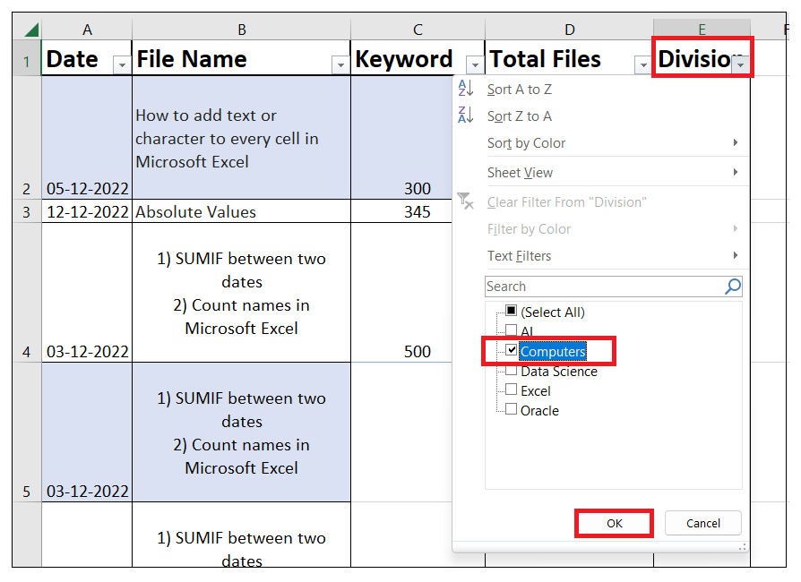
For example, here we have filtered data the rows only for computers course to view the content for this.

That's it! You are done! Applying filter is that easy in Microsoft Excel.

How to filter blank / non-blank cells

While working with Excel, the blanks cells are one of the major crises that commonly we need to filter out. Whether you want to filter blanks or non-blanks, do one of the following:

To filter out blanks, click on the filter dropdown, and the following window will appear, make sure the Select All box is checked, and last uncheck the Blanks field present at the bottom. It will show only those rows containing values in the selected column.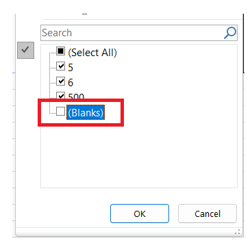

To filter out non-blank cells (to show only the cells containing nothing), uncheck the Select All box and select the Blanks field. It will show all the blank cell rows in the selected column.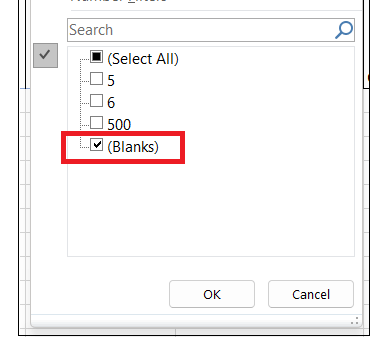

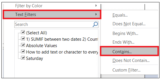
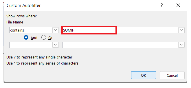
If you wish to delete the Blank columns from your worksheet, you must filter out the non-blank cells. Select the filtered output, right-click on them, and click the Delete row option.

Notes: The Blanks option will only be available if the selected columns contain at least one empty cell.

How to add Filter for different data values

Let's cover the steps to filter data on the basis of text and number values.

Filter Text Data

Text data is one of the most commonly used datatypes in Excel. When you filter text, by default, Microsoft Excel provides some options that will ease the text filtering process. Those options involve: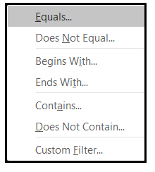

• Filter cells that are equal to or completely match the given text.
• Filter cells that are not equal to the given text value.
• Filter cells that begin with the given text value.
• Filter cells that ends with the given text value.
• Filter cells that contain the specified value anywhere in the text.
• Filter cells that do not contain the specified value anywhere in the text.
• You can opt for the custom filter to create your filter options if none of the above suits your requirements.

For example, below given are the steps to filter out rows containing SUMIF text:

1. Go the Data tab, click on Filter option present under Sort & Filter group.
2. Click on the filter icon on any of the column header where you want to apply the Text Filters.
3. The window will appear, select the Text Filters option, and along with that select the required filter. In our case, we have selected Contains....
   
4. As shown below, the Custom AutoFilter dialog box will appear. Type the text value for which you want to create the filter or you can select it from the from the dropdown list.
   
5. Once done click on OK button.

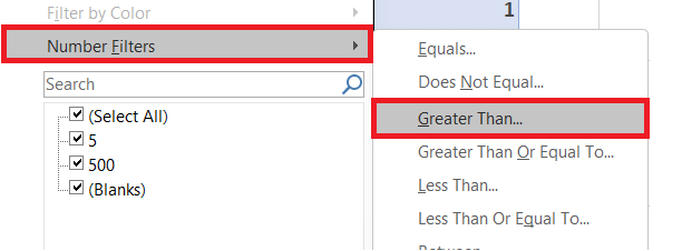
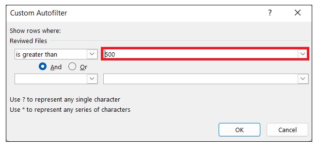
Filter numbers in Excel

Unlike Text values, you Excel provides different options to filter the numeric data as well, it includes: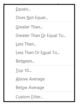

• Filter cells that are equal to or completely match the specified number.
• Filter cells that are not equal to or completely match the specified number.
• Filter numbers that are greater than, less than or lies between the given number.
• You can also easily filter the top 10 or bottom 10 numbers.
• Filter the cells on the basis of above average or below average.

For example, below given are the steps to filter out rows containing value greater than 300:

1. Go the Data tab, click on Filter option present under Sort & Filter group.
2. Click on the filter icon on any of the column header where you want to apply the filter.
3. The window will appear, select the Number Filters option, and along with that select the required filter. In our case, greater than....
   
4. As shown below, the Custom AutoFilter dialog box will appear. Type the number value for which you want to create the filter or you can select it from the from the dropdown list.
   
5. Once done, click on the OK button.

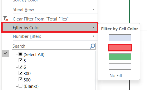
How to filter by color in Excel

If you have formatted your data using conditional formatting, in such cases you can filter the data by color as well. You can apply the filter with respect to cell color, font color and cell icon.

Microsoft Excel provides a default option to filter by colour. Click on the auto-filter drop-down arrow, and in its window, and it will show the options to Filter by Color (where the options depend on the formatting you have applied to the selected column):

For instance, we have formatted the cells using a combination of two colours, i.e., red and green. You can show only the red cells using the Filter by the colour option. Perform the following steps to get it done:

1. Apply the conditional formatting to the any of the column.
2. Go the Data tab, click on Filter option present under Sort & Filter group.
3. The filter arrow will appear on all the header cells, click on the filter icon.
4. From the resulting list, select the Filter by Color option.
5. Select the required color - red in our case.
   
6. As a result, Excel will only display the cells with red conditional formatting. You will have the following output.

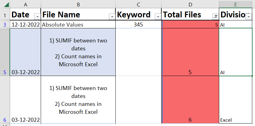
How to filter in Excel with search

The Excel filter option includes a search box that is extremely helpful for navigating large data sets. Using this field box, you can quickly filter rows by entering the exact name, date, number or text.

For instance, in our case, we want to display all the records containing all the data about the Excel course. All you need to do is to click on the filter icon. Look for the search box from the resulting dropdown and type the word Excel. As a result, the Filter panel will instantly match the record from the column data and quickly present all the items that match the search. To view only the rows containing Excel data, press the enter key or click on the button.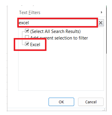

If you want to extend the filter for multiple searches, you must type the second search field. Once the result appears, check the box for Add current selection to filter option, and click on the OK button. For example, we are adding AI to the already filtered 'Excel' data list.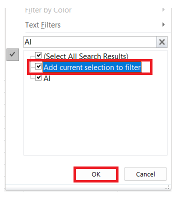

Excel will return the following filtered output: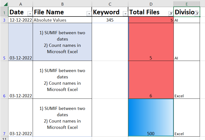

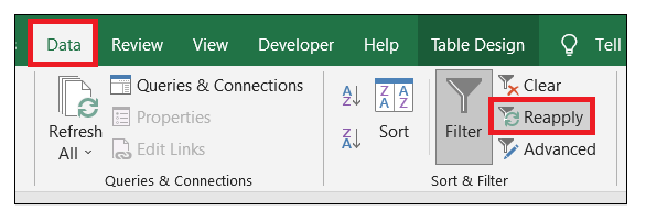
Re-apply a filter after changing data

Many times, after applying the filter we edit or delete something from the filtered cells. But the problem after doing such edits is that Excel AutoFilter does not update those changes automatically. To reflect them, you need to re-apply the filter by using the following steps:

• Put your cursor anywhere within your dataset.
• Go to the Data tab, from the Sort & Filter group, click in Reapply option

OR

• Go to the Home tab, From the Editing group, click on Sort & Filter-> Reapply.

How to copy filtered data in Excel

So far we have covered how to filter different data. Now the question arises how to copy and paste the filtered data to another worksheet? The steps are simple and easy to implement. All you need to do is to follow the below shortcuts:

1. Put your cursor on any of your filtered cell, and press the shortcut key Ctrl + A. It will select all the filtered data including the table headers.
   If you don't want to copy the column headers of the filtered data, select the first (upper-left) cell, and after that, press the shortcut key Ctrl + Shift + End to expand the data selection to the last filtered cell.
2. Press the shortcut key Ctrl + C to copy the data.
3. Spot your cursor to the cell destination or switch to another sheet/workbook, and press the shortcut key Ctrl+V to paste the filtered data.

Note. For small datasets, the above shortcuts work perfectly fine where the filtered data is only copied. But sometimes, while working with large workbooks, the hidden data or the filtered-out rows are also copied (though it happens in rare cases). To prevent such situations, select the filtered range of data cells and press the shortcut key Alt + ; it will select only visible cells ignoring the filtered-out rows. Or else you can also take advantage of the Excel Go To Special feature (Go the Home tab. From the Editing group, click on Find & Select option > Go to Special... > Visible Cells only).

How to clear filter

Once you have filtered your data, make the invisible data visible. To enable so, all you need to do is to clear all the filters to make the data visible again.

To clear the filter from a specific column, click on the filter icon and from the window then click on 'Clear Filter from <Column name>'. Refer to the below image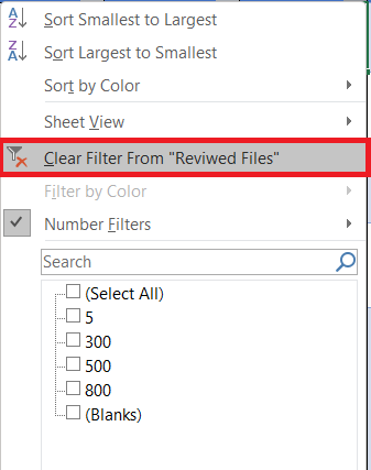

Doing so will remove the filter from the respective column.

Remove filter from Excel worksheet

Perform the following steps to quickly remove all filters from your existing worksheet:

Click on the Data tab, go to the Sort & Filter group, and click on Clear option.

OR

You can go to Home tab > Editing group, and from the resulting options click on Sort & Filter > Clear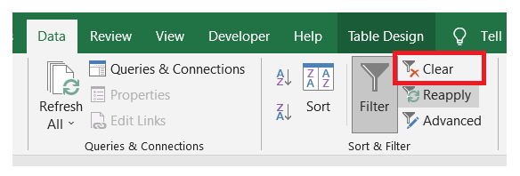

Filter not working in Excel

Many times, the AutoFilter fails to give the required output or stops working halfway down a worksheet. Though these situations commonly occur if the filter is not applied properly or sometimes it occurs because some new data has been entered outside the range of filtered cells in your worksheet. To fix the above problem, you can perform one of the following solutions:

1. Re-apply the filter to the cells.
2. If re-applying the filter doesn't work, use the clear all option and apply the filters from start.

That's it for this tutorial! But unlike in Excel, advancement is all you need, give the above options a try, and you can go deeper with filters.