How to do subtraction in Excel?

With Excel, users get an option to record vast amounts of data sets. Although it enables users to record almost all data types, numbers are the most commonly used data within the cells in an Excel worksheet. Since Excel is spreadsheet software, it allows performing calculations between the recorded data sets. Subtraction is one of the four primary arithmetic operations and is most often used in Excel.

In this tutorial, we discuss various step-by-step methods or solutions on how to do subtraction in Excel. We discuss a few step-by-step methods for subtracting between data based on use cases, including related example data sets.

How to subtract in Excel?

Unfortunately, there is no definite SUBTRACT function like Excel's SUM function. However, Excel has several alternate methods we can use to do subtraction within the worksheet. We may have to try different approaches depending on how the data is organized and how we want to subtract the desired data. Let us now explore some commonly used subtraction methods in Excel:

Subtracting Values in a Cell (Minus Formula)

We all know that subtraction is one of the easiest arithmetic calculations in mathematics. We can also use the subtraction concept in an Excel sheet, like in math. In math, we use the equal sign after the subtraction formula. However, in Excel, we use the equal sign before the subtraction formula within the cell.

The basic Excel subtraction formula is defined as below:

We can apply the above formula in an Excel cell using the below steps:

• First, we must type an equal (=) sign in the resultant cell where we want the subtraction result to appear.
• Next, we need to enter the first number, a minus sign, and the second number.
• Lastly, we must press the Enter key on the keyboard to record the formula result.

We can use more than one arithmetic operation in an Excel cell, which allows us to subtract multiple numbers simultaneously within the cell.

For example, suppose we want to subtract 15 from 95; the basic subtraction equation to use within the cell will be like this:

=95-15

To subtract multiple numbers from a specific number, we can enter all numbers similarly to the above equation by separating them by a minus sign. We can also insert the parentheses for complex arithmetic calculations to obtain results correctly.

The below image shows some subtraction formulas within Excel cells and their corresponding results: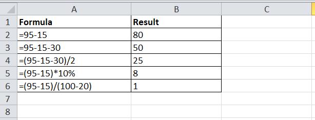

Subtracting between Different Cells

It does not make sense to subtract between different numbers directly in Excel. We often perform calculations between the cells which contain the respective numbers. So, it is essential to know the subtraction method between different cells.

When we need to subtract one cell from another, we use the same concept as the previous method. However, we enter the corresponding cell references in the generic formula instead of the numbers. The basic Excel subtraction formula to subtract the numbers between two different cells is defined as below:

We can apply the above formula in an Excel cell using the below steps:

• First, we must select the cell to record the subtraction result and type an equal sign (=) to begin the formula.
• Next, we need to type the cell address containing the first number. We can also click on the specific cell via the mouse, and the respective reference (or address) appears within the formula automatically.
• After that, we must type the minus (-) sign and type or select another cell containing a number to be subtracted.
• Lastly, we must press the Enter key to retrieve the subtraction output.

For example, suppose we want to subtract the number recorded in cell B2 from the number in cell A2, the basic subtraction equation to use within the cell will be like this:

=A2-B2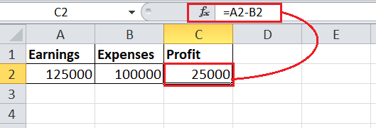

Subtracting Cells in Different Columns

When we need to subtract cells in different columns for several cells of individual rows, it will be difficult to apply the subtract formula multiple times using the previous method. However, Excel provides a simpler way to perform subtraction for multiple cells in different columns. We only need to apply the subtraction formula in the top-most cell for the cells in a row and drag or copy the same in the remaining cells below in the resultant column.

For example, suppose we have multiple earnings data in column A and corresponding expenses in column B, and we need to calculate the profit (or subtraction result) in the respective cells of column C.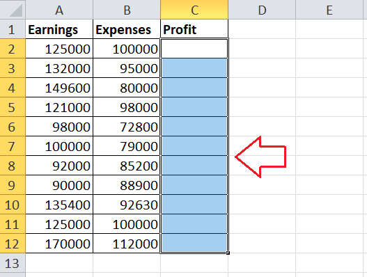

Although we can apply the subtraction formula between cells in each corresponding cell of column C one by one, it is not a convenient way. Instead of applying the subtraction formula between cells multiple times, we only apply this in the first resultant cell of column C, i.e., cell C2. The following formula calculates the profit (subtraction result) for the example data in the second row (similar to the previous method we discussed):

=A2-B2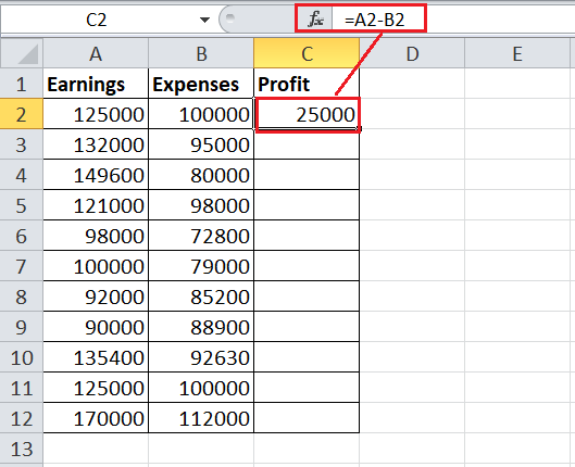

After subtracting cells in different columns of the second row, we drag the effective formula by holding the 'Fill Handle' from the bottom-right corner of the formula cell.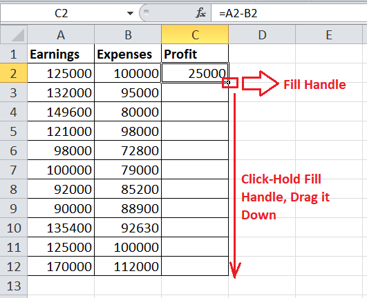

Since Excel uses relative cell references by default, the formula automatically adjusts the cell references for each of the following rows accordingly.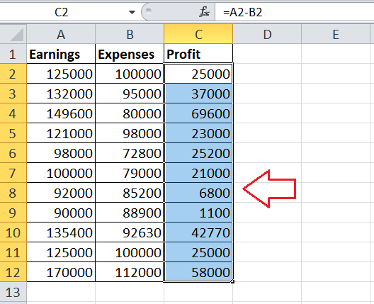

Subtracting One Specific Cell (Number) from Entire Column

Unlike the previous method, suppose we only need to subtract one cell from a range of cells of any specific column. In that case, we cannot simply insert the formula in the first cell and copy (or drag) to others. Due to the relative cell references, the formula will change the reference for the specific numbers of cells accordingly, leading to the wrong result.

For example, let's consider the following sample data where we have month-wise earnings in column B. We need to deduct a fee of 2000 rupees (recorded in cell E2) from each cell of column B to calculate the profit (or subtraction result) in the corresponding cells of column C.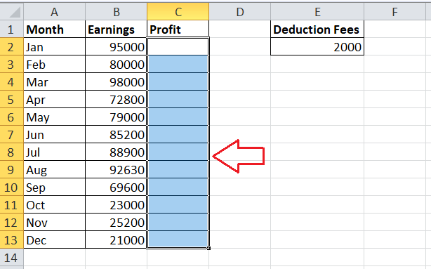

The simplest method to calculate the profit is subtracting the number 2000 from the top-most earning cell in C2 and copying it down to other cells. The formula will look like this:

=B2-2000

After we copy the above formula from C2 to other cells till C13, the cell references will adjust automatically due to relative referencing. However, this is not an efficient method if we need to change the deduction fees again and again. We have to edit the formulas accordingly.

Instead of subtracting the number from a cell, we can subtract between the responsible cells. But, we have to lock the cell reference for the cell to be subtracted. Thus, we create an absolute referencing that doesn't change automatically after copying it.

Since the deduction fee is a fixed number, we need to lock only cell E2 (a cell containing the deduction fee). As a result, our effective subtraction formula to use in the first resultant cell C2 becomes this:

=B2-$E$2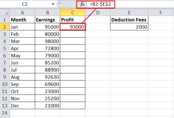

After copying (or dragging using the Fill Handle) this formula to other cells in column C, the relative cell references for the cells in column B change automatically. However, the cell E2 remains locked (or absolute) since we used the dollar sign to fix its row and column address.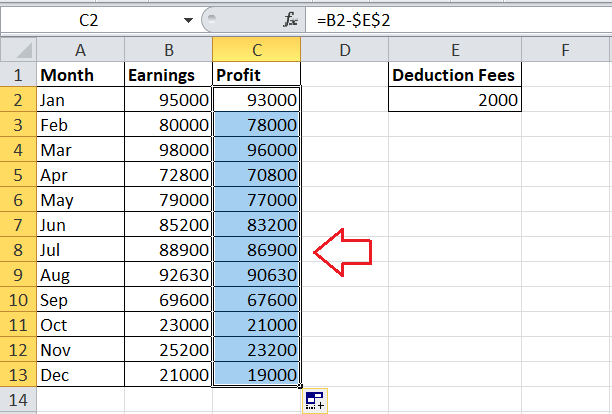

If we now change the deduction fee in cell E2, the results in all of the corresponding cells in column B will automatically update in a real-time.

Subtracting Multiple Cells from One Specific Cell

If we need to subtract multiple cells from any specific cell in the Excel worksheet, we can choose any of the following three options:

By Using the Minus Sign

The basic way to subtract multiple cells from the same cell is to type their cell references separated by minus signs. It can be referred to as the combined Minus Formula.

For example, suppose we need to subtract cells from B2 to B5 (B2:B5) from cell B1. We can use the Minus Formula and include the effective cells in the following way:

=B1-B2-B3-B4-B5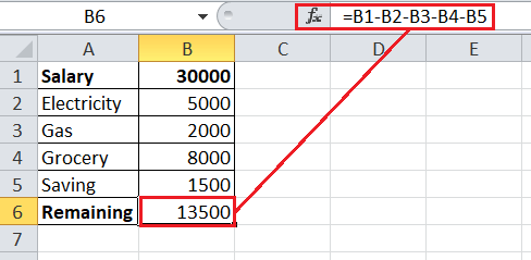

By Using the SUM Function

In maths, we usually add all the negative numbers and then subtract the addition results by the positive number to get the effective output. The same concept can be used in Excel when subtracting multiple cells from any specific cell. So, we use the SUM function to add up all the numbers to be subtracted and then subtract the result from the primary cell (or number).

In our example sheet, we can insert the following SUM formula to subtract the cells B2:B5 by B1:

=B1-SUM(B2:B5)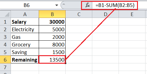

By Using the Negative Numbers

Another typical method for subtracting multiple cells from a single cell involves using the same mathematical concept we applied in the previous SUM function formula. Accordingly, we explicitly add negative signs before the numbers in all cells we want to subtract. Afterwards, we must apply the SUM function to the entire range to add the negative numbers with the positive number cell from which we wanted to subtract.

In our example, we insert the minus sign in cells B2:B5 and then construct the SUM formula in the following way:

=SUM(B1:B5)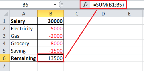

Subtracting Dates in Excel

In Excel, the dates are evaluated as integers. No matter how we format the dates in an Excel cell, their corresponding integer or the numeric form is interpreted by Excel in the backend. Excel typically calculates the numbers for the dates by counting the day's gap from the starting date supported in Excel, i.e., January 1, 1900.

For example, if we type the date January 01, 2021, in an Excel cell, its integer form will be 44197 as 44197 days have passed from the starting date to the entered date.

Because of the generic numbers evaluation of dates in Excel, it is easy to subtract one date from another. We can easily find the difference between two specific dates and calculate how many days have passed between them.

The most straightforward method to subtract the dates in Excel is to enter them in different cells and then subtract between them using their cell references. However, it is essential to note that we must always use the end date first in the formula to avoid negative dates output.

The basic subtraction formula to subtract between two dates is defined as:

Consider the following sample data set where we have 'Start Date' and the 'End Date' in columns A and B, respectively. We need to calculate the number of days (or subtraction results) between the recorded dates in different columns.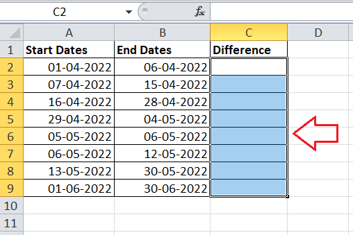

Thus, we apply the basic subtraction formula in our first resultant cell, C2, like this:

=B2-A2

Afterwards, we copy or drag the formula into other corresponding cells in column C.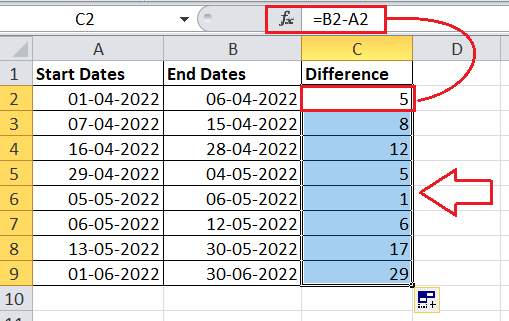

Sometimes, we may see the dates even after the subtraction in the resultant cells. In such cases, we have to change the cell format of the resultant cells from 'Date' to 'General' by navigating to the Home tab > Number drop-down list > General. This will display the dates in numbers, making it easier for us to know the difference in days between the given dates.

Subtracting Time in Excel

Similar to dates, the times are also evaluated as numbers by Excel. However, unlike the dates, the times are stored as decimals in the backend, not as integers or whole numbers.

For example, if we type the decimal number 44197.5 and convert it to time, Excel will convert it to January 01, 2021, 12:00 PM. Likewise, 44197.25 would represent January 01, 2021, 09:00 AM.

Therefore, no matter how the times are visible or formatted within the cells, they are just decimals numbers. So, the subtraction between times is also possible in Excel.

We can subtract between cells containing the time using the following basic equation:

If we have the example data set with start and end times in columns A and B, respectively. We can apply the subtraction formula in the first resultant cell of column C (C2) like this:

=B2-A2

Afterwards, we copy the above formula in the other remaining cells of column C to differentiate time outputs.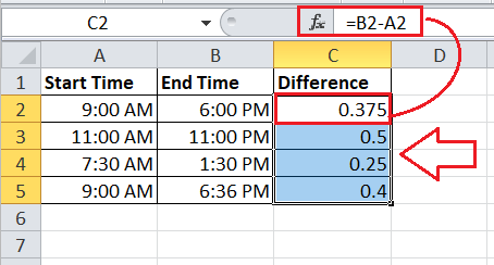

If we see a time format in our resultant cells in column C, we must select these cells and convert them to General by navigating to the Home tab > Number drop-down list > General.

Although the time differences are calculated, the output does not make much sense in decimals. We can convert these decimals to hours, minutes and seconds to make them more meaningful. For that, we need to multiply the decimal numbers in the resultant cells by 24 (for getting hours), 24*60 (for getting minutes) and 24*60*60 (for getting seconds).

So, if we multiply our difference decimals in example data sets by 24, we can determine how many hours elapsed in the resultant difference.

=(B2-A2)*24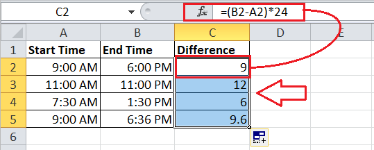

Subtracting Percentages in Excel

When we need to subtract one percentage value from another within an Excel cell, we can usually put those percentage values in the cell with a minus sign between them. This creates the Minus formula for the percentages. However, we must ensure to start the formula with an equal sign (=) in an Excel cell.

For instance, we can insert the below formula to subtract the one percentage value of 30 from another percentage value of 100:

=100%-30%

Alternatively, we can record these percentage values in different cells (suppose A2 and B2) and subtract them using their cell references.

=A2-B2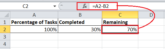

The subtraction process becomes a little difficult when we need to subtract a percentage value from any specific number instead of another percentage value. In that case, we need to use the below generic formula:

It is often used to decrease any number by any desired percentage value. We can supply the percentage value directly in the formula or use the respective cell reference.

For example, suppose we have employees' salary data in column A, and we need to decrease the salary by 10% for some reason. In that case, we can enter the percentage value in another individual cell (i.e., B2) and use the below formula using the relative references for the number (salary) cells and absolute reference for the percentage cell:

=A2*(1-$B$2)

Afterwards, we drag the above formula into the remaining cells of the resultant column C. The relative references will change accordingly for each respective salary data while the percentage cell remains locked. So, we get the desired subtraction percentage results accordingly.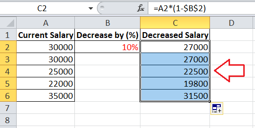

Important Points to Remember

• It is recommended to always use the highest or the largest number as the first argument in the subtraction formulas to avoid negative results.
• When subtracting dates or times, we must ensure that input data is in the same corresponding formats before applying the formulas to subtract between them. The subtraction formulas will return errors if the data is given as text strings.