HLOOKUP formula in Excel

HLOOKUP is a "Horizontal lookup" to search the value in the topmost rows. It is an Excel function, which helps the users to search and retrieve the data from the topmost row in an Excel worksheet. This function runs a bit differently than the other Excel functions.

In the name of HLOOKUP, "H" refers to Horizontal. It means that the searching and retrieve operations are performed horizontally on rows moving to the right. Hence, HLOOKUP is also known as Horizontal LOOKUP.

Note: Unlike the MATCH() function, it does not return the position of the matched item; it returns matched value.

HLOOKUP() is a sibling to the VLOOKUP() method. It looks for the value according to the topmost row within the defined range. Basically, it performs two (search and retrieve) operations on the heading of the Excel data.

Uses of HLOOKUP

Like the MATCH() function, HLOOKUP() also supports exact and approximate matches of data. Besides that, it also supports the wildcards (*, ?) operators for the partial matching on Excel data.

The users can use these operators to perform partial matching on data. It looks for the data within the defined range and row.

Syntax and parameters

HLOOK() function consists of four parameters, and here is the syntax for it:

Here, the first three parameters are mandatory and LOOKUP_range is an optional one.

Parameter list

These parameter values of the HLOOKUP() are separated by comma.

Return value

1. The HLOOKUP() function returns the value to which the user is looking for.
2. If the value is not found within the specified detail, it returns a #N/A error. The #N/A refers to the Value Not Available

Important points to be remembered

Following are some essential points to be remembered while performing the HLOOKUP() function on your Excel data.

• HLOOKUP is a case-insensitive Hence, Orange and ORANGE both are the same for it.
• The first parameter (LOOKUP_value) should contain a value from the topmost row. Or we can say that it must be one of heading of the table.
• HLOOKUP function support for wildcard characters (*, ?) in the LOOKUP_value parameter for the partial match of data.

Errors generated by HLOOKUP() function

The HLOOKUP function generates an error if the specified value matches the criteria. These errors are -

1. #N/A error
2. #VALUE! error
3. #REF! error

#N/A error

If the value is not found within the specified detail, it returns the #N/A error. The #N/A refers to the Value Not Available error.

#VALUE! error

If the row_index parameter consists of value less than 1, i.e., row_index < 1. LOOKUP() returns the #Value! error. The #VALUE! refers to the Error in Value error.

For example, range_index is 0 or less than 0.

#REF! error

If the row_index is greater than (>) the number of columns in table parameter, i.e., row_index > 1. LOOKUP() returns the #REF! error. The #REF! refers to the Invalid Cell Reference Error error.

Remember that - HLOOK() will return only one value or error at a time.

An Example with formula

Let's understand with the help of syntax example.

=HLOOKUP("Headphones",B1:G10,5,0)

Here,

• Headphones is the value of one of the columns heading we are looking for.
• B2:H9 is the range in your Excel worksheet within which we are looking for data.
• 5 is the row number in which the value will be searched.
• 0 is optional, but here specified for the exact match of data.

How to perform HLOOKUP() on your Excel worksheet?

HLOOKUP function executes differently than the other Excel functions. Let's consider an example to understand the working of the HLOOKUP() function.

We have some electronics sell data of 7 days (1 week) in an Excel worksheet. We will now use the HLOOKUP() function to find a particular electronic sell of a specific day. In this way, it will help us to find the data from the large dataset very easily.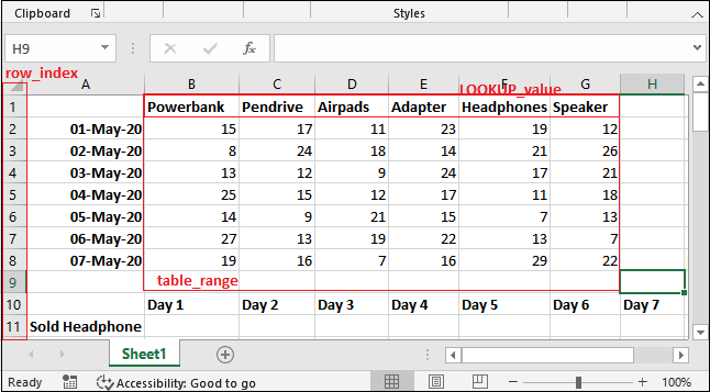

See the steps below:

Example 1

We will find the one-day sell of headphones. In this example, we look up the day 3 sell of headphones. For this, follow some easy steps for the HLOOKUP formula:

Step 1: Select a cell to store the outcome and write the HLOOKUP formula in such a way, as shown below:

=HLOOKUP("Headphones",B1:G8,4,0)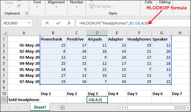

Step 2: Get the total number of headphones sold on 4^th May by pressing the Enter key and see that it returned 11. It means that total 11 headphones have been sold on 3^rd May.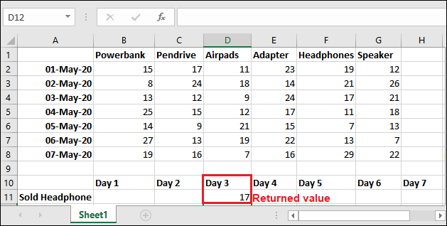

You can verify that the HLOOKUP formula is working properly or not by finding the data manually. See below how to verify this: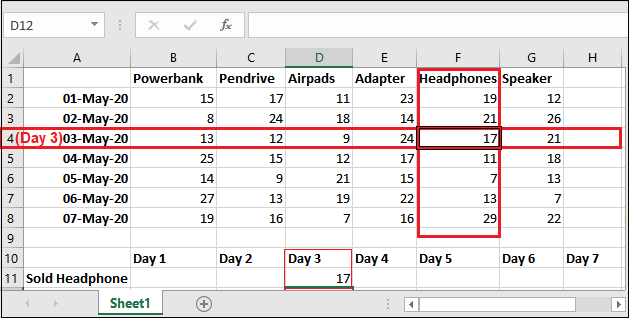

Error Message Example

Following are three different examples for each error (#N/A, #REF, #VALUE) generated by the HLOOKUP(). These errors with their examples are described below.

Example 1: When exact match not found - #N/A error

As we already discussed with you that the HLOOKUP() function returns the #N/A error if the value is not found within the specified detail. The #N/A refers to the Value Not Available error.

See an example for it below:

Step 1: You can see that we are looking the Headphone inside the HLOOKUP() formula with an exact match (0) parameter value. But in the Excel table, the heading is Headphones, which is not the same.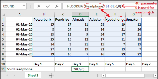

Step 2: Once you write the formula (=HLOOKUP("Headphone",B1:G8,6,0)) for the value whose exact match is not available and press the Enter key, you will get #N/A error.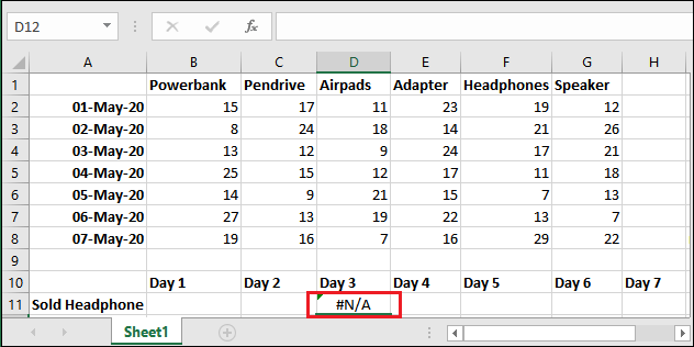

Example 2: When row_index > selected range (table) - #REF! error

The HLOOKUP() function returns the #REF! error if the row index parameter value is greater than the number of columns selected in the table parameter.

See an example for it below:

Step 1: You can see that we have selected a range for table parameter between B1:G8 in HLOOKUP() formula, i.e., till Row 8. But we are looking for row_index 9, which does not come within the defined range.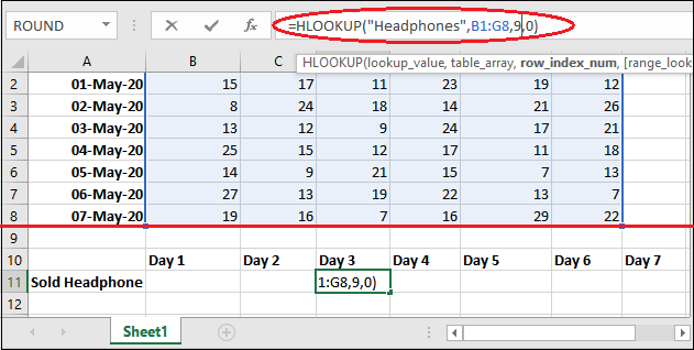

Step 2: Once you write the formula (=HLOOKUP("Headphone",B1:G8,9,0)) where row_index is higher than the selected range and press the Enter key, you will get #REF! error as showing below.

Example 3: When row_index < 1 - #VALUE! error

The HLOOKUP() function returns the #VALUE! error if the row index parameter value is less than the 1 in the targeted Excel worksheet.

The #VALUE! refers to the Error in Value error.

See an example for it below:

Step 1: You can see that we have selected a range for table parameter between B1:G8 in the HLOOKUP() formula. But we are looking for row_index = 0, which is less than 1, i.e., the row is not available in the Excel worksheet.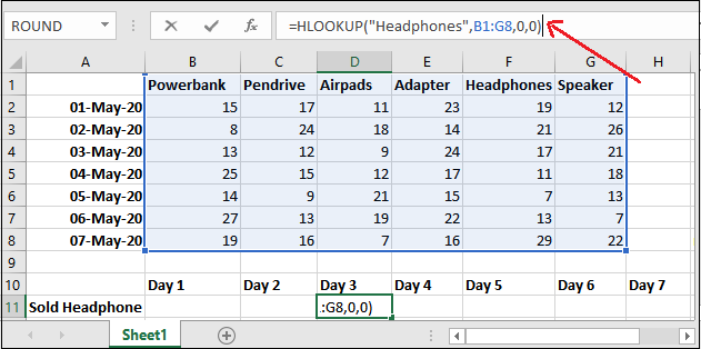

Step 2: Once you write the formula (=HLOOKUP("Headphone",B1:G8,0,0)) where row_index is less than 1 and press the Enter key, you will get #VALUE! error as showing below.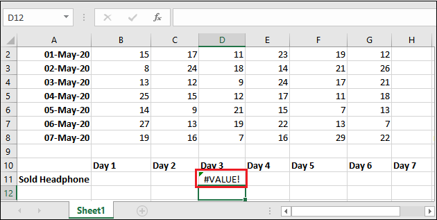

Use of wildcards in HLOOKUP()

HLOOKUP function can use wildcard operators. We will use the same Excel workbook in its example below -

Step 1: We will look for the sell of the fourth day for the product whose name starts with P. For this, use asterisk (*) operator with the first parameter and copy the below formula:

=HLOOKUP("P*",B1:G8,5,FALSE)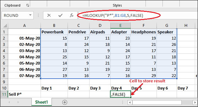

We used FALSE in the 4^th parameter for the exact match.

Step 2: Now, by pressing the Enter button, get the 4^th day sell of a product whose name starts with P.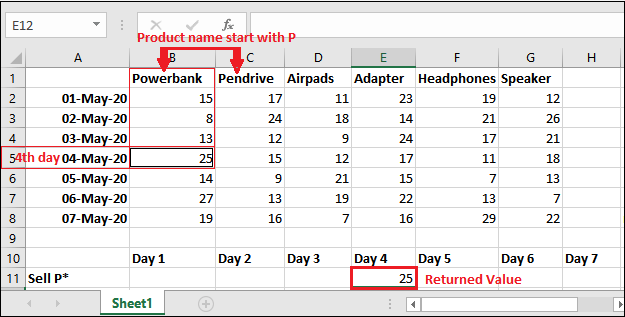

It returned the value of the fourth day when it finds the first product, whose name starts with P. See the above result.

Similarly, you can use another wildcard operator in it.