Excel Creating Formulas

MS Excel, short for Microsoft Excel, is a widely used powerful spreadsheet program that provides access to different worksheets in a single workbook. Users can store large amounts of data in these worksheets using existing cells. One of the significant advantages of using Excel is that it allows us to perform various calculations, operations, and analyses. Excel has a wide range of pre-defined functions, and we can perform almost every operation in Excel by creating formulas through existing functions.

In this tutorial, we discuss the various step-by-step methods of creating formulas in Excel properly. The steps for creating or using a formula differ for each Excel function as each function requires different arguments. However, the basic concept remains the same. Before we discuss the methods of creating a formula, let us briefly understand the definition of an Excel formula.

What is the Formula in Excel?

An Excel formula is nothing but an introductory statement consisting of one or more 'operands' and 'operators'. The formulas in Excel help us specify the relationship between the values recorded within the cells in the worksheet, perform mathematical calculations on the recorded values, and retrieve the desired results in a resultant cell.

One essential point to note while using the formulas in Excel is that we must always start them with an equal sign (=). If we don't start the formulas with an equal sign, they are not treated as formulas but only as a text string.

The Difference between a Formula and Function

An Excel formula is a statement or an equation structured manually by a user to perform any calculation. At the same time, the Excel function is the pre-defined calculation in the spreadsheet program. We can use more than one function in a formula.

Example of Formula: =A1+A2+A3

Example of Function: =SUM(A1:A3)

How to create a formula in Excel?

There are several methods we can use to create formulas in Excel. We discuss the most common methods below, and each method has its advantages. All of the following methods for creating formulas work in all versions of Excel.

Creating Formulas using Constants and Operators

When creating formulas in Excel, constants are numbers, dates, or text values involved within the formula. In addition, the operators are any sign, symbol, or character that refers to an action or operation to be performed. The most common arithmetic operations include addition, subtraction, multiplication, division, exponentiation, and modulus operations.

To create a basic Excel formula in an Excel cell using the constants and operators, we must perform the steps below:

• First, we need to select a cell to record the output or result.
• Next, we must type an equal symbol (=) and enter the formula equation to perform the calculation.
• Lastly, we must press the Enter key on the keyboard to obtain the results.

Creating an Excel formula using constants and operators is different from writing an equation in maths. The fundamental difference is that we start the formula with an equal sign in Excel, while in mathematics, we usually insert an equal sign at the end.

For example, if we want to add two numbers (3 and 5), an Excel formula will look like =3+5. However, in maths, we use 3 + 5 =. When we insert an Excel formula in an Excel cell and press the Enter key, the result of the formula appears like the following image: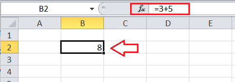

Creating Formulas using Cell References

Instead of typing the numbers directly into the Formula equation, we can also refer to the corresponding cells that contain the required numbers (or values) in the sheet. It is more convenient and easier to use cell references in formulas when working with large data sets. Furthermore, one advantage of using a cell reference is that the formula results are automatically updated in real time whenever we change the value in the corresponding cell/range.

To create a formula using the cell references, we can perform the below steps:

• First, we need to select a cell to record the output.
• Next, we enter the equal sign (=). After that, we need to type the first cell that contains the number. It is not mandatory to always type the cell reference. Instead, we can also click on the specific cell, and Excel will automatically fetch the cell reference of that cell in the applied formula. This eliminates human error.
• In the next step, we must type the operator sign we want to apply for the formula. For example, if we want to sum up the first and second cell values, we must use the addition sign (+) between them.
• After entering the operator sign, we need to type the cell reference of another number that we want to include in our formula.
• Lastly, we must press the Enter key to obtain the formula result.

Suppose our example sheet contains two numbers, 3 and 5, in the cells A1 and B1. We need to calculate the sum of these values in cell C1 using the formula containing cell references. So, we have to apply the following formula in a cell C1:

=A1+B1

After we press the Enter key, the result will appear in a cell C1, as shown below: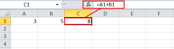

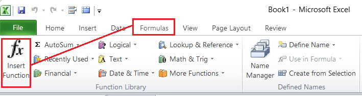
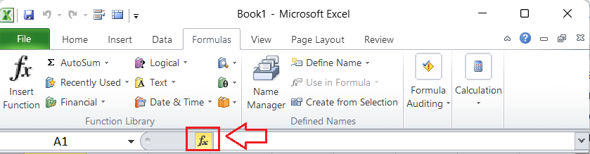
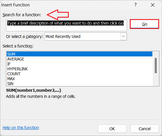
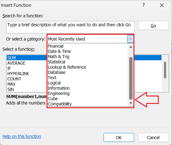
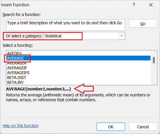
If the values are recorded in more than two cells, we can use the cell reference of each cell similarly. For example, if we have values in cells A1, B1, and C1, we can add their corresponding values using the formula =A1+B1+C1. However, if several cells are required in a formula, it is better to try using existing functions and ranges of cells.

Note: By default, Excel uses relative references and changes them accordingly when copied from one cell to another. If we need to prevent them from automatically changing by Excel, we must use absolute references. To switch between references, we must press the F4 function key on the keyboard.

Creating Formulas using the Pre-defined Functions

When there are multiple cells to use in the formula, and if they are contiguous, it is even better to use the entire range than to use each cell reference separately. Using the range in Excel helps us save time and get the desired results more accurately. Additionally, we can also use the cell references in formulas when combining the equation through functions.

No matter the function name, the formula still begins with an equal sign followed by the function name and the required arguments enclosed within the parenthesis. However, each function has a different syntax structure and requires specific arguments. We must know the syntax, necessary arguments, and the order of the function we want to use.

When creating a formula by combining the existing Excel functions, we usually have two common ways. We can either use the function wizard to select the desired function (s) in our formula or directly type/ write the entire formula with the functions into a cell or formula bar. Let us discuss both the ways of creating formulas in Excel:

Using the Function Wizard

Using the Function Wizard to create a formula in Excel is the most trusted and effective way. If we find creating formulas complex or are beginners in Excel, the Function Wizard comes real handy. To create a formula in Excel using the Function Wizard, we must go through the following fundamental steps:

• First, we need to select a resultant cell by clicking on it and running the Excel function wizard. We need to navigate the Formulas tab and click on the 'Insert Function' button under the 'Function Library' section, which will launch the 'Insert Function' window.
  
  Alternatively, we can also use the 'fx' button from the left side of the formula bar to insert the desired function in a cell.
  
  Another quick way to insert a function in Excel involves using the function drop-down list. After selecting the cell, we must type an equal sign (=) and choose the function from the drop-down list present to the left of the formula bar.
  
  
• In the Insert Function window, we typically get the three options using which we have to find and select the desired function. We have to type the function name in the first option box and click on the Go button. Additionally, we can type the desired function's description or operation and click 'Go' to find relevant function names. However, it is not such a convenient option if we don't know the appropriate name of the function.
  
  When we are not sure of the function's name, we must manually select the category to which our function may belong. The list has about 14-16 different categories, and all the existing Excel functions are divided into them accordingly.
  
• After selecting the category of the desired function, we will see a list of various functions under the section 'Select a function'. We need to find the desired function in the list, and we can select the function in the list to get more information about it. Excel will display the information or description with the syntax of that particular function we selected.
  
• Once the function name is found, we must click the OK button. This will launch the 'Function Arguments' window, where we need to pass the desired or required arguments/ parameters for the function. When entering the arguments for any function, Excel shows all the required information in the window. We can type the cell (s) or a range manually in the respective boxes or use the selection box icon from the end of the box to select the cells in the sheet using mouse clicks.
  
  In the above image, we can see that the result also appears at the bottom of the window after we pass/ select the desired arguments for the function.
• Lastly, we must click the OK button or press the Enter key on the keyboard to complete the formula and retrieve the corresponding formula result in a selected resultant cell.
  

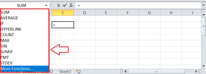
Typing/ Writing a formula into a Cell or formula bar

It seems a lengthy process, although it is easy to create Excel formulas using the Function Wizard. If we have knowledge about the Excel function we want to use, a faster way would be to type it directly into the cell or formula bar and pass the corresponding arguments according to the formula syntax.

As usual, we first have to select a cell to record an output value. Next, we must enter the equal sign (=) followed by the desired function name. When we start typing the function name into an Excel cell, a list with the relevant function names appears in front of us. We can also select the desired function from the list by pressing the TAB key on that particular function. When we write the function name manually, we must manually type the starting parenthesis sign. However, a starting parenthesis is automatically inserted when selecting a function from the list by pressing the TAB key.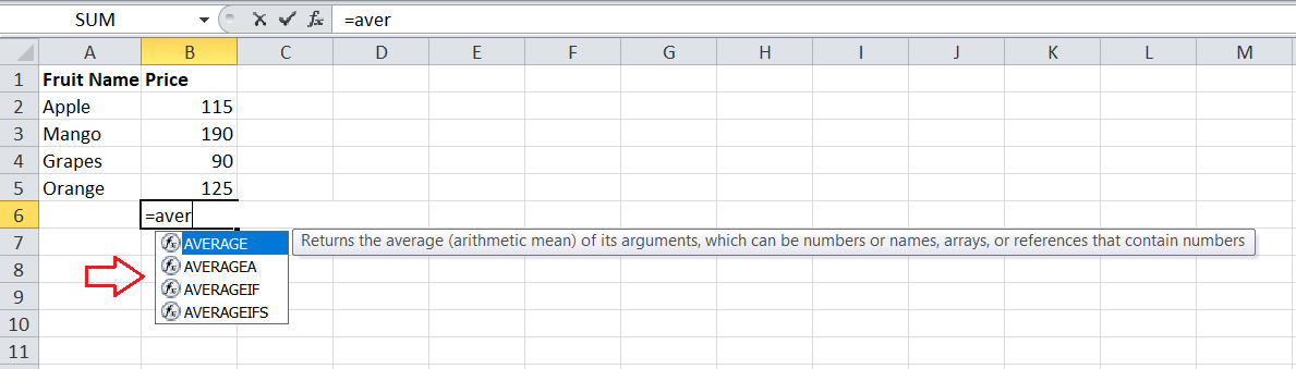

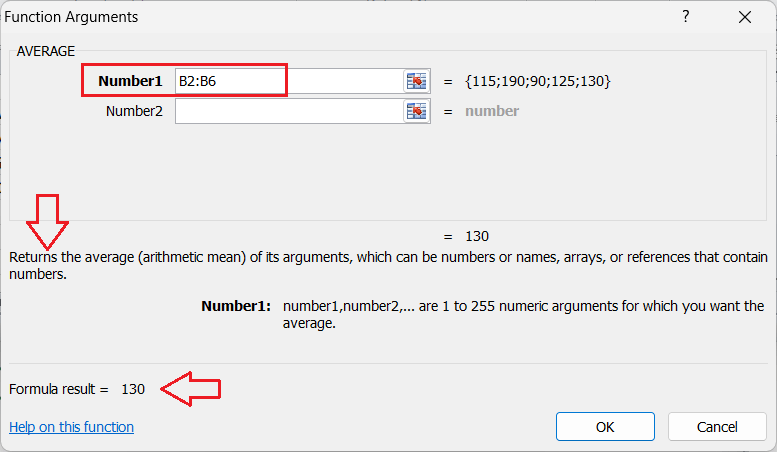
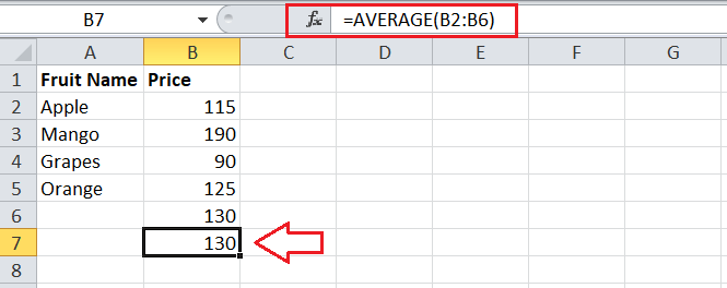
As soon as we write/ select the function name, Excel automatically shows the syntax for that function, highlighting the arguments required for the function. We can type the cell reference or a range manually or click on the specific cells/range to include them in our formula.

For example, the following image shows the formula to calculate the average price for the recorded values in cells from B2 to B5.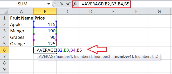

In the above image, we used each cell reference separately. However, we can also use the range B2:B5 instead of repeatedly typing/selecting each cell. We can easily cover large data sets in our Excel formula by supplying an entire range.

Lastly, we must type the closing parenthesis and press the Enter key to get the final results.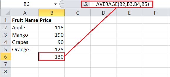

When we have data in different worksheets that we want to include in the formula, we must also specify the sheet name with the range of cells when writing the cell references manually. For example, suppose we have numbers in a range B2:B5 in two different sheets, Sheet1 and Sheet2. In that case, we can use the following formula and calculate the average:

=AVERAGE('Sheet1'!B2:B5,'Sheet2'!B2:B5)

In contrast, if we select the cell reference by clicking on the corresponding cell, the sheet name is automatically inserted in the formula by Excel.

Note: It is recommended to use the Function wizard instead of directly writing the function into a cell. By selecting a function from the function wizard, we can reduce the chances of Excel errors.

Creating Formulas using Defined Names

Instead of using the cell references/ ranges in the formula directly, we can also specify a desired name for the specific cells/ range and use it later in our formula. However, it will not be easy for others to understand the formula.

For example, suppose we name the two cells A2 and B2 as Revenue and Expenses, respectively. We can use the below formula in another cell to record the 'Net Income' by subtracting the expenses from the revenue:

=Revenue-Expenses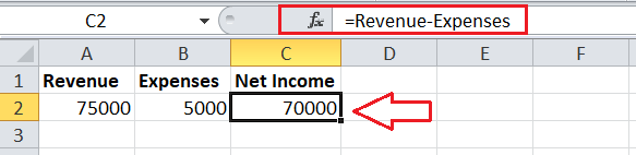

Here, we defined the names of cells. However, we can also define a name for the entire range, usually called Named Range.

To manage (define, view, edit, or delete) any name for the cell(s) or a range, we must go to Formulas > Name Manager. However, the fastest way to define a name in Excel is to select the specific cell (s)/ range and type the desired name directly in the Name Box, where we usually see the cell reference.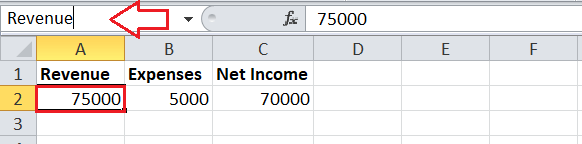

Important Points to Remember

• In Excel, we can copy formulas from one cell to another cell in the same worksheet, another sheet, and even in another workbook. However, we must be careful while copying the formula as the cell references may change unexpectedly.
• If we delete any row/column or cell containing the formula's value, the formula result may change to #REF! error. In that case, the function treats the deleted cell/row/column as an invalid reference and gives an error.