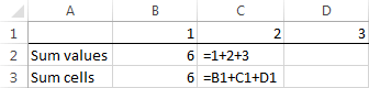
How one can make use of the SUM Function in Microsoft Excel

It was well known that the respective "Sum function" is the other most important mathematical function that can be used, for the purpose of summing up all the selected numbers, whether it could be a decimals number or whole numbers. And we can also either select the cells which are containing the numbers one by one or directly we can select the complete range of the cells whose Sum we need to find out respectively.

SUM Formula in Microsoft Excel:

The respective that can be used for the purpose of "SUMMATION" of the cell in Microsoft Excel are as follows:

FORMULA:

=SUM (number1,[number2],....)

The numbers like 'num1', 'num2', and 'num_n 'basically denote the numeric values or the numbers which we wish to add on.

And it can also accept numbers up to 255 or individual arguments in a single formula.

How to Sum in Microsoft Excel by making use of the simple arithmetic calculation?

We can make use of the Microsoft Excel as a mini calculator if we need a quick total of the individual cells, and need to utilize the plus sign operator (+) as in a regular arithmetic operation of the addition.

• For example: 1) Adding of values none other than: 1,2,3
  2) Adding of cell: B1, C1, D1

Moreover if we want to sum a few hundred rows, then in that scenario, referencing each cell in a formula does not sound like a good idea.

How we can make use of the SUM function in Microsoft Excel

The Microsoft Excel SUM function is primarily mathematics as well as the trigonometric function which are responsible for adding up the values.

And in our Excel SUM formula, every argument can be: positive value as well as the negative value, or it could be in the form of the range respectively.

• For example:

=SUM (A1:A100)

=SUM (A1, A2, A5)

=SUM (1,5,-2)

The Excel SUM function is very much helpful when we are required to add on the values from the different ranges, or we can easily combine numeric values, cell references, and ranges as per our requirement.

• For example:

=SUM (A2:A4, A8:A9)

=SUM (A2:A6, A9, 10)

The below screenshot shows these and a few more SUM formula examples respectively: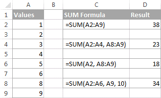

And in the real-life sheet Microsoft Excel "SUM function" is often included in bigger formulas as part of the more complex calculations.

• For example: In this one can easily embed out the SUM in the value_if_true argument of the IF function for the purpose of adding out the numbers in columns B, C, and D if all three cells in the same row contain values, as well as show a warning message if any of the cells are blank respectively:

=IF (AND ($B2<"", $C2<>"", $D2<>""), SUM ($B2:$D2), "Value missing")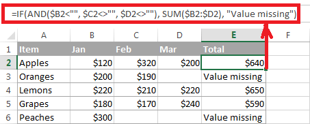

How one cans easily AutoSum in Microsoft Excel?

If in case we are required to sum one range of the numbers, whether it could be a column, row then we can let Microsoft Excel to write an appropriate SUM formula for us efficiently.

And for this, we will select a cell next to the numbers which we want to add; after that, we will click on the AutoSum that are present just under the Home tab, and in the Editing group, we will press the Enter key from our keyboard.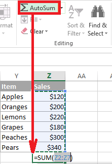

It is clearly visible from the above screenshot that the Microsoft Excel's AutoSum feature will not only enters a Sum formula but also it will selects out the most likely range of cells which we do not want to be in our total. The Excel will get the range right there nine times out of ten.

And apart from calculating the total, we can make use of the AutoSum features to automatically enter out the various functions which are none other than the: AVERAGE, COUNT, MAX, or MIN.

How we can sum a column in Microsoft Excel?

Now to sum numbers in a given specific column, we can use either the Excel SUM function or the AutoSum feature.

• For example: If we want to sum values in column B, that is from cell B2 to B8, we are required to enter the following Excel SUM formula as well:

=SUM (B2:B8)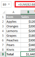

Totaling of an entire column with an indefinite number of rows in Excel sheet

Let us assume that, we are having a column which we want to sum and it has a variable number of rows, which means that the new cell can be easily added while the existing ones can be deleted at any time. So in that particular case, we can easily sum out the entire column by just supplying a reference without specifying a lower or upper bound.

• For example =SUM (B: B)

Important note: And it should be noted that in no case we should put our 'Sum of a column formula in the column in which we want to total it because of the reason that this would create a circular cell reference and our Sum formula would be returning 0 in this case respectively: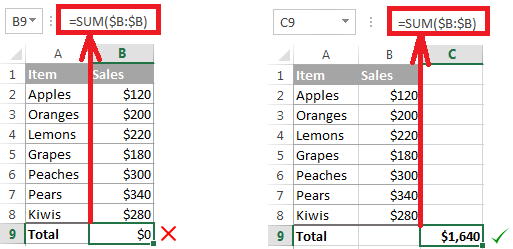

Sum column except for header or excluding a few first rows

And we all knew that, supplying a column reference to the respective Microsoft Excel Sum formula will totals out the entire column while just ignoring the header. But sometimes, the column header which we want to total can have a number. Or, we could exclude the first few rows with the respective numbers irrelevant to the data we want to sum out.

Furthermore, the respective Microsoft Excel will not accept a mixed SUM formula with an explicit lower bound but an accept without an upper bound, and now, if we want to exclude the first few rows from summation, then we can make use of the following workarounds as well.

• Summation of the entire column and after then will subtract out the cells which we do not want to include in the total.

=SUM (B: B)-SUM (B1:B3)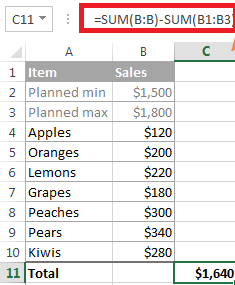

Moreover, it should be remembered that the respective worksheet size should have the limits, and we can easily specify the upper bound of our Excel SUM formula that are based upon the maximum number of rows used in our Microsoft Excel version.

• For example: To sum column B without the header (i.e., excluding cell B1), we can make use of the following formulas as well:

1. In Microsoft Excel version 2007, Microsoft Excel version 2010, Excel 2013, and Excel 2016:
   =SUM (B2:B1048576)
2. And in Microsoft Excel version 2003 and lower:
   =SUM (B2:B655366)

How can one Sum rows in Microsoft Excel?

Similar to the totaling of a column, we can quickly sum out a row in Microsoft Excel by using the SUM function, or we can also use the AutoSum to insert the formula for us effectively.

• For example: For the purpose of adding out the values in the respective cells that are B2 to D2, we can make use of the following formula as well:

=SUM (B2:D2)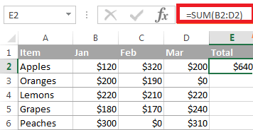

How can we sum out the multiple rows in Microsoft Excel?

Now to add values in each row individually, we can drag down our Sum formula as well. And the main point which needs to be remembered is to make use of the relative references (without $) or mixed cell references (where the $ sign fixes only the columns).

• For example:

=SUM ($B2:$D2)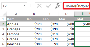

And to total out the values in a given range that are containing several rows, we are required to specify out the desired range in the Sum formula respectively:

How can the Microsoft Excel Total Row sum data in a table?

Let us now assume that, our respective data is organized in an Excel table. In that case, we can benefit from the unique Total Row feature, which can quickly sum out the data in our selected Table and display the totals in the last row.

Furthermore, one of the most significant advantages of making use of the Microsoft Excel tables is that they auto-expand new rows, so any new data we input in a table will be get automatically added in our formulas as well.

And if we want to convert a normal range of the cells into a given table, we can select it and will then press out the shortcut Ctrl + T shortcut (or click Table on the Insert tab) as well.

How can one add a total row in Microsoft Excel tables

After the arrangement of the data in a selected table, we can easily insert a total row in this way as well:

1. Firstly we will be clicking anywhere in the Table to display the Table Tools with the Design tab.
2. And on the Designtab, which is present under the Table Style Options group, we will be selecting the Total Row box:

And the other way can be used to add a total row in Microsoft Excel is to right-click any cell within the given Table, and then will be clicking on the Table> Totals Row.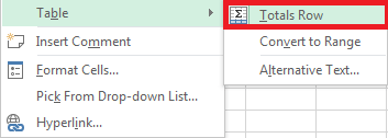

How can one perform totaling of our data in our Table in Microsoft Excel?

It was well knew, that the respective total row get appears just at the end of the Table, and Microsoft Excel does its best for the purpose of determining out how we would like to calculate data in the selected Table as well.

As in our sample table, the values which are present in the column D (rightmost column) will be get added automatically, and the Sum will be displayed in the Total Row: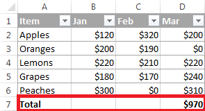

And to total the values in other columns, we are required to select a corresponding cell in the total row; after that, we will be clicking on the dropdown list arrow and then will select the Sum formula respectively: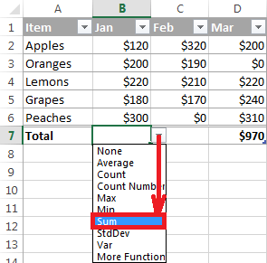

If we want to perform another calculation, we will select the corresponding function from the dropdown list, like Average, Count, Max, Min, etc.

And if in case the total row get automatically displays out a total for a respective column that does not need one, just open the dropdown list and will select the none option from it.

How can one easily sum only filtered (visible) cells in Microsoft Excel

Some of the time we are required to filter or hide some out some of the data in our separate worksheets for more effective data analysis. A usual Sum formula would not work in this case; this is because of the reason that the Microsoft Excel Sum Function will add up all the values in the given specified range, that will includes out the hidden (filtered out) rows as well.

And if in case want to sum only and only the visible cells in a filtered list, then the fastest way is to just organize our data in Microsoft Excel table and then turn on the Excel total row feature available in the sheet as well.

Besides this, the other way which can be used for the Sum filtered cells in Microsoft Excel is to apply an AutoFilter to our data manually by just clicking on the Filter button present on the Datatab. And then, write a Subtotal formula by ourselves.

The SUBTOTAL function has the following syntax:

SUBTOTAL (function_num, ref1, [ref2],)

In which,

• Function_num: It is a number which are ranging from 1 to 11 or 101 to 111, and it will specify out the function which can be used to the subtotal as well.

Here in this, we are quite interested only in the SUM functions which are usually defined by the numbers which are ranging from 9 to 109. And both the numbers will exclude out the filtered-out rows. But the main difference is that the number 9 will primarily include manually hidden cells (i.e., right-click > Hide), while 109 excludes them.

And if in case we want to only sum visible cells, irrespective of how exactly the irrelevant rows were hidden, in that case, we can make efficiently make use of the number 109 in the first argument of our Subtotal formula.

• Ref1, Ref2 ...: It is termed to be the cells or ranges which we want to subtotal, and the very first Ref argument is required.

How does one efficiently perform running total (cumulative Sum) in Microsoft Excel?

Now for the purpose of calculating a running total in Microsoft Excel, we can write a usual SUM formula with the clever use of the two references that are none other than absolute as well as the relative cells references.

• For example: To display out the cumulative Sum of the respective selected numbers in column B, we will be entering the following formula in cell C2 and then will copy it down to other cells as well:
  =SUM ($B$2:B2)

And the relative reference B2 will be getting changed automatically that are based upon the relative position of the row in which the formula is copied efficiently: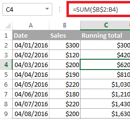

How can one sum across sheets in Microsoft Excel?

Now in this, if we are having a several worksheets and that with the same layout, the same data type, in that scenario, we can easily add out the values in the given same cell or in the same range of cells in the different sheets with the use of the single SUM formula respectively.

And a so-called 3-D reference is what does the trick:

=SUM (Jan: Apr! B6)

Or

=SUM (Jan: Apr! B2:B5)

Now the first formula will usually add on the values in the selected cell that is B6, while the second formula will sum out the range from cell ranging from B2:B5 in all worksheets that are located in between of the two boundary sheets which we have specified (Jan and Apr in this example):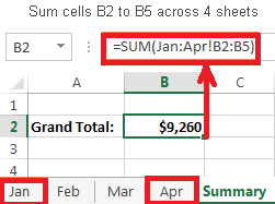

Microsoft Excel conditional sum

If in case, our respective task requires adding of only those cells that will meet a particular condition or a few conditions, then in that case we can effectively make use of the SUMIF or SUMIFS function.

• For example: The following SUMIF formula will eventually add only those amounts in column B in which we have "Completed" status in column C:
  =SUMIF(C: C,"completed", B:B )

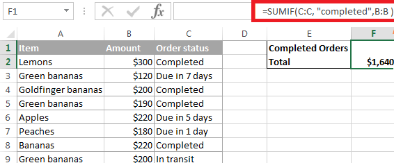
And in order to calculate out a conditional sum with the multiple criteria, we can just make use of the SUMIFS function. As we have used it in the above example, for the purpose of getting the total of "Completed" orders with an amount over $200, and we can make use of the following SUMIFS formula as well:

=SUMIFS (B: C:C,"completed",B:B, ">200" )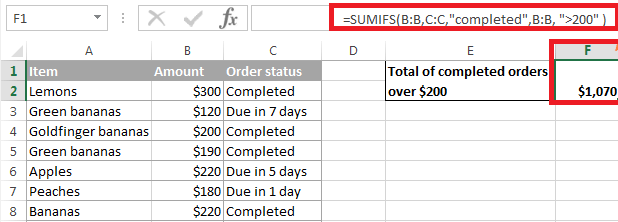

Important Note: It should be noted, that the Conditional Sum functions are made available in the Microsoft Excel versions that usually begin with Excel 2003 (more precisely, SUMIF function was rarely introduced in Excel 2003, while SUMIFS was only in Excel 2007.

Microsoft Excel SUM not working - reasons and solutions

Are we trying to add a few values or total a column in our Microsoft Excel sheet, but a simple SUM formula only computes some of it? And if in case the Microsoft Excel SUM function is not working properly, then it is most likely because of the following reasons which are mentioned below in details.

1. #Name error appears instead of the expected result

It is one of the most accessible errors to fix. As in 99, 100 cases, the #Name error will indicate that the SUM function is misspelled.

2. Some of the numbers are not added properly

And the other common reason for a Sum formula (or Excel AutoSum) not working is that the numbers are formatted in the form of text values. At first sight, they will look like a normal numbers, but Microsoft Excel will perceives them as text strings and leaves them out of calculations.

3. Excel SUM function returns 0

Apart from the numbers that are basically formatted in the form of the text, a circular reference is considered to be the common source of the problems in case of the Sum formulas, mainly when totaling a column in Microsoft Excel. So, if our numbers are formatted in the form of the numbers, but our Excel Sum formula will still return a value of zero, then in that case we need to trace and fix out the circular references in our sheet (Formula tab > Error Checking > Circular Reference).

4. Excel Sum formula returns a higher number than expected

If, against all expectations, our respective Sum formula returns a more significant number than it should be remembered that the SUM function in Microsoft Excel will efficiently add on both the visible as well as the invisible (hidden) cells respectively.

5. Excel SUM formula not updating

And when a SUM formula in Microsoft Excel continues to show the old total even after we have updated the values in the particular dependent cells, most likely the Calculation Mode is set to Manual as well, and to fix this, we can go to the Formulastab, and then will be clicking on the dropdown arrow which is present next to Calculate Options, and then will be clicking on the Automatic option respectively.