Consolidate data in Excel

Data consolidation is a very interesting and useful feature of Excel. It helps the user to gather the data together from different worksheets and collect them in a master workbook. In this way, it allows the users to take the data together. Data in a single table is easy to update.

Consolidate is an Excel function that let the users to collect the data from different locations and summarize it into one Excel table. The main trouble with the data consolidation method is that it is a bit tricky to work with data consolidation. This chapter will guide you step by step to use data consolidation.

Ways to consolidate data

In MS Excel, you can consolidate the data in two ways, either by category or position.

Consolidate by category

When the data in all source sheets/workbooks is not arranged means not in order but uses the same labels (row and column heading), consolidate the data by position. This method can be used to consolidate the data from multiple worksheets, which have different layouts but the same data labels.

Consolidate by position

Consolidate the data by category when the data in the source worksheets has the same order and also uses the same labels. Use it to consolidate the data from multiple worksheets.

For example, departmental budget worksheets created using the same template.

Important point

Consolidating data by category is the same as creating the pivot table. When the pivot table is created, a user can easily recognize the category. You can choose to create a pivot table if you want more flexible consolidation by category.

What we can do with consolidate data?

An Excel user can do the following by the use of data consolidate -

1. Consolidate data from multiple worksheets and collect it in the same workbook
2. Consolidate data from multiple workbooks and put it into a new workbook

Hence, we will show you the example for both of these cases. Continue with this chapter below.

Before moving forward, you must know that the following processes will work with the newer version of Excel (versions above Excel 2007). If you are using a lower version from Excel 2007, it will not work.

Where is consolidate option is present?

To consolidate the data, you can find the Consolidate option inside the Data tools section. This Data tool section is available inside the Data tab in the Excel ribbon. E.g.,

Data tab > Data Tools section > Consolidate feature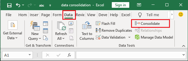

Consolidate data from multiple worksheets within the same workbook

We have three sheets in an Excel workbook containing three years of expenditure on tea, coffee, and cold drink (on a quarterly basis). All three sheets are named Year1, Year2, and Year3, respectively. Means that - each worksheet contains a year of data and it is broken down into quarters.

To consolidate the data within the same workbook, we can insert a new worksheet in the same workbook and name it as Consolidate Summery. This consolidated summery sheet will show the expenditure by year and quarter.

See our three of worksheets for year1, year2, and year3 with data is as follows -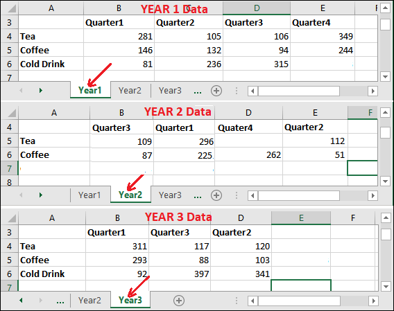

It does not matter that all three worksheets data is arranged in the same order (same arrangement of columns and rows). Excel will automatically arrange them for the users while consolidating.

In this screenshot, you can see that all three years (1, 2, and 3) have different arrangements of rows and columns.

• Cold drink row does not have value for quarter4 in year 1 sheet.
• Year 2 worksheet does not have the row of cold drink and these quarters are also arranged in a different order.
• There is no quarter4 in year3. So, the number of rows and number of columns are different in all three sheets.

Still, you can consolidate the data in a separate sheet within the same workbook.

Steps to consolidate data

To consolidate the data, you must first to insert an empty worksheet to make it a master sheet to keep the data after consolidation.

Step 1: Insert a new worksheet within the same workbook. Renamed it as Consolidate Summery to make it easily recognizable.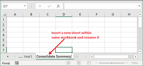

Step 2: Inside consolidate summery worksheet, select the first cell or any other where the consolidated data will appear.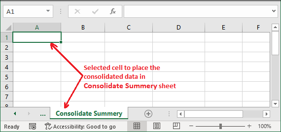

Step 3: Go to the Data tab in the Excel ribbon and click the Consolidate button inside the Data Tools section.

Step 4: A consolidate dialog box will open like below, provide the value and select the options you require.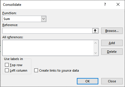

1. Select the function based on which you want to consolidate the data. E.g., SUM. You can select SUM inside the function dropdown list to consolidate data.

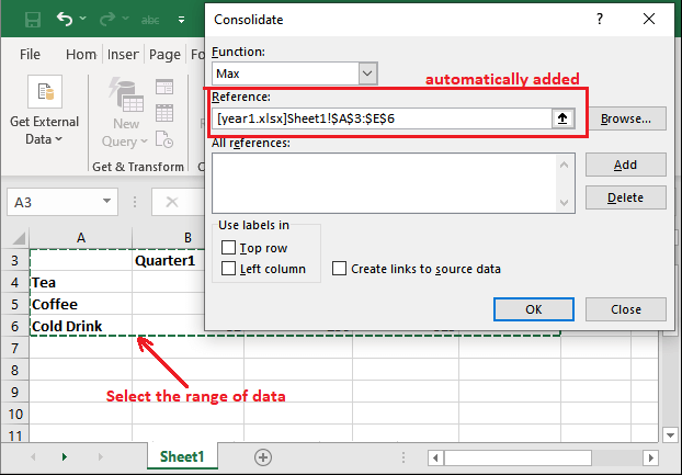
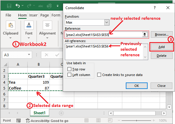
2. In the Reference area, select the first data ranges of sheets one by one to consolidate.

a. Keep the cursor on the reference area and go to the targeted sheet, i.e., Year1, without closing the consolidate panel.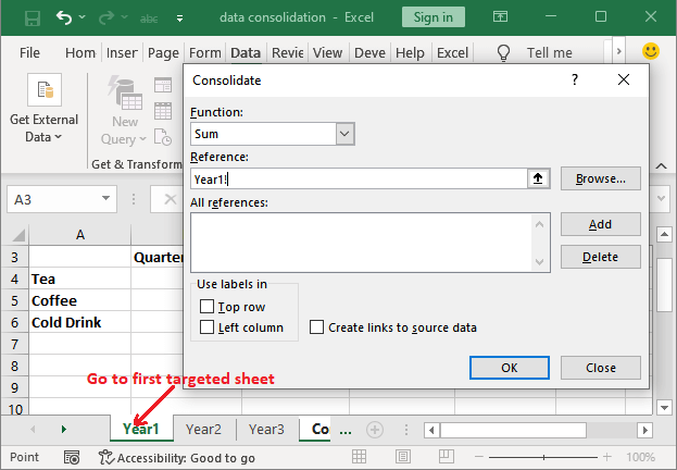

b. Now, select the range of data over here (including both headers) to add for consolidation.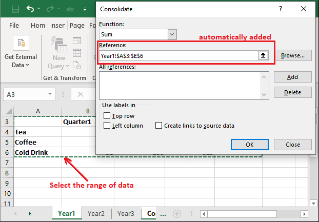

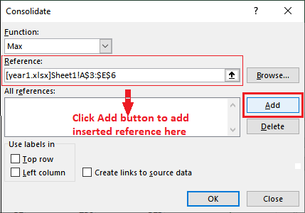
You will see that the selected range is automatically added to the reference field.

c. Now, click the Add button to add this first set of data to the All References area in consolidate dialog box.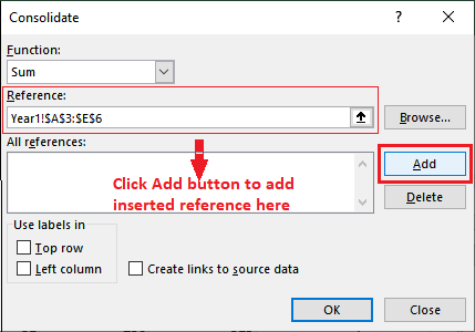

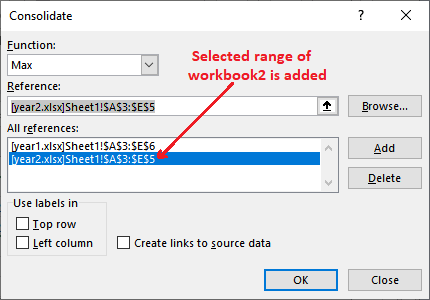
d. Now, navigate to the Year2 worksheet and select the range as in the above steps. After that, click the Add button to move it into all references field.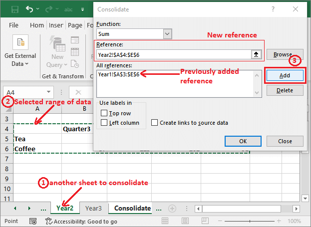

e. See that another reference is added here.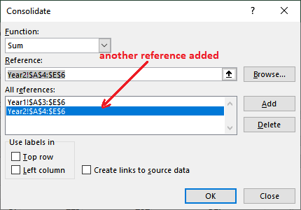

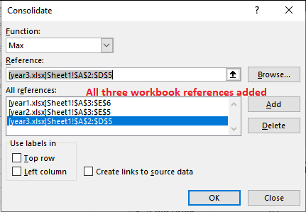
Continue the same process for other worksheets to add them in consolidate dialog.

f. See that all three of them sheets range of data is added to inside the References field. Now, click the OK button here.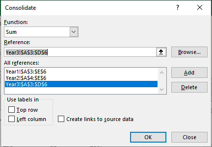

Tip: You can also provide the name to the targeted range of data of each data before start consolidate process so that you can recognize them easily.

3. To indicate that where the labels are located in source ranges, consolidate has two checkboxes: Top Row and Top Column. Mark them accordingly.

4. Our data has a row header (Quater1, Quater2, Quater3, Quarter4) and column header (Tea, Milk, Coffee), so mark both checkboxes.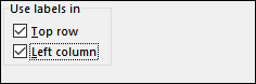

5. Mark the Create links to source checkbox if you want automatic update in the consolidate sheet on changing in source data.

Step 5: When all settings are done, you can now click the OK button.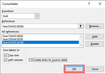

Step 6: Your data will be pasted inside the consolidate summery sheet (newly added sheet) within the same workbook.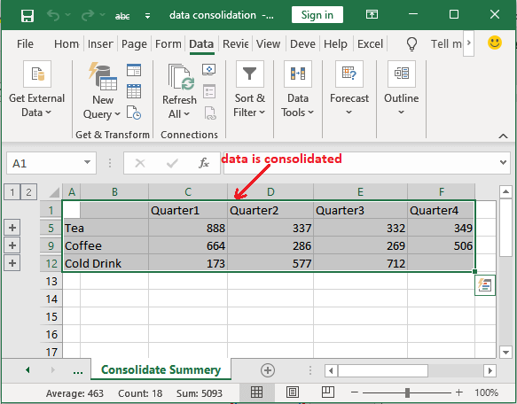

Read out the consolidate summery

After consolidating the data, you must need to understand how this data is merged/consolidated. So, we will help you out with this. You remembered that you had chosen the SUM function. So, the resultant data for each year is summed up together and pasted in consolidate worksheet.

Step 7: On the left side of the Excel screen, you will find grouping tools (+), which you can use to expand and hide the data.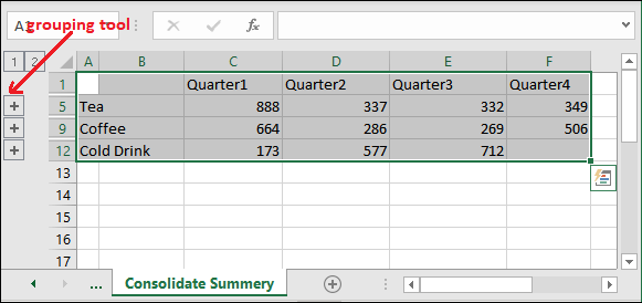

Step 8: Click the first grouping tool (+) to expand and see how the consolidated result is calculated for the Tea row.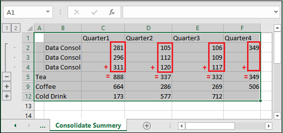

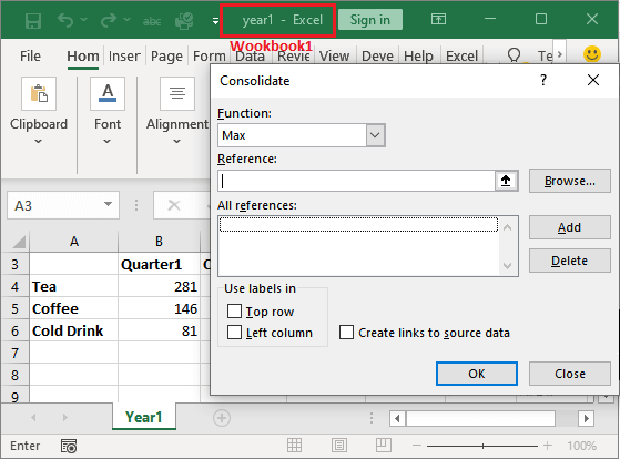
For tea row -

Quarter1: 281+296+311 = 888

Quarter2: 105+112+120 = 337

Quarter3: 106+109+117 = 332

Quarter4: 349 = 349

Similar to this, consolidated data is calculated for other rows data. When you expand the grouping tool for the corresponding row, you will find it.

Consolidate data from multiple workbooks to a new workbook

This time, we have data in different workbooks instead of one from which we will collect together and consolidate in a new workbook. It contains the expenditure on tea, coffee, and cold drink for three years in separate workbooks broken down into quarters.

To consolidate the data in a new workbook, the Excel users has to create a new Excel same workbook and name it Consolidate Summery. This consolidate summery workbook will show the expenditure by year and quarter.

See our workbook data in three of workbooks for year1, year2 and year3 are as follows -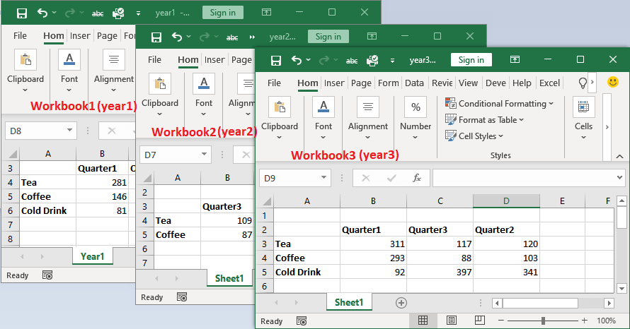

This type of consolidation requires when the user have data in different workbooks instead of one. In such a scenario, the Excel users can use consolidate data from different workbooks to a new workbook.

Three of the workbooks contain data in a different order and cold drink row in year2 workbook and quater4 column in year3 workbook are also missing. No need to be worried; Excel will automatically arrange them for you while consolidating the data. It might be possible that they do not have the same number of rows and columns in all three workbooks. Still, you can consolidate the data in a separate workbook.

Steps to consolidate data from different workbooks

To consolidate the data in a new workbook from different workbooks, you have to first create a new Excel workbook that will keep the consolidated data.

Step 1: Create a new Excel workbook and save it by the name Consolidate Summery.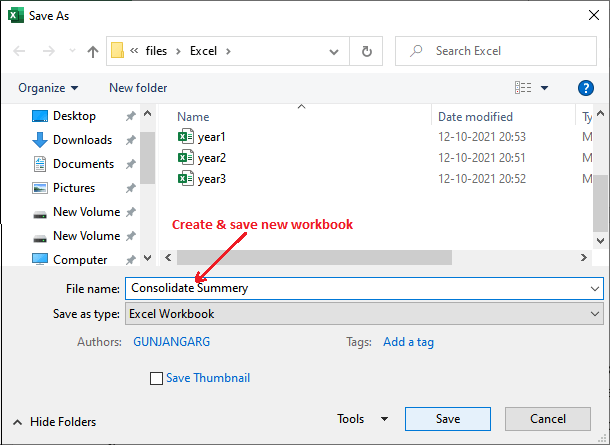

Step 2: Inside the newly created workbook, select a cell where the consolidated data will appear and go to the Data tab in the Excel ribbon.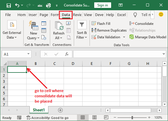

Step 3: Click the Consolidate button inside the Data Tools section.

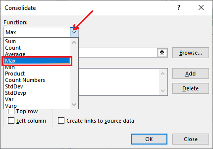
Step 4: A consolidate dialog box will open like below, provide the value and select the required options.

1. Firstly, select the function based on which you want to consolidate the data. E.g., SUM, MAX, MIN.
   We will select MAX inside the function dropdown list to consolidate data.
   
2. In the Reference area, select the first data ranges of sheets one by one to consolidate.
   1. Keep the cursor on the reference area and go to the targeted Excel workbook, i.e., Year1, without closing the consolidate panel.
      
   2. Now, select the range of data of this workbook along with both headers to add it for consolidation.
      
      Your selected data range of workbook1 is added in the reference column on the above selection.
   3. Now, click the Add button to add this first set of data to the All References area in consolidate dialog.
      
   4. In the second workbook (year2) and select the range as in the above steps. After that, click the Add button to move it into all references field.
      
   5. See that another reference is added here.
      
      Continue the same process for other worksheets to add them in consolidate dialog.
   6. See that all three of them sheets range of data is added to inside the References field. Now, click the OK button here.
      
3. To indicate where the labels are located in source ranges, consolidate has two checkboxes: Top Row and Top Column. Mark them accordingly.
4. Our data has a row header (Quater1, Quater2, Quater3, Quarter4) and column header (Tea, Milk, Coffee), so mark both checkboxes.
   
5. Mark the Create links to source checkbox if you want automatic update in the consolidate sheet on changing in source data.
   

Step 5: When all settings are done, you can now click the OK button.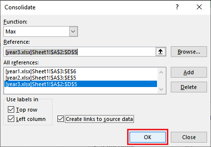

Step 6: Your data will be pasted inside the consolidate workbook (newly created workbook) as consolidate summery.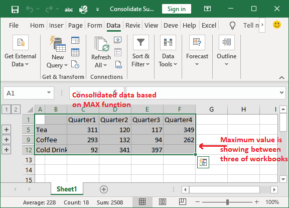

Your data is consolidated based on the MAX function. So, now each row cell contains MAX value between all three years of workbooks for each quarter.

Analyze the consolidated data

After consolidating the data, you should how this data is consolidated understand how this data is merged/consolidated. So, we will help you out with this. You have remembered that you had chosen the MAX function. So, the resultant consolidated summery sheet shows the max value for each cell by comparing three of the workbooks data.

Step 7: On the left side of the Excel screen, you will find grouping tools (+), which you can use to expand and hide the data.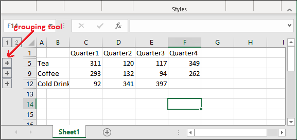

Step 8: Click the first grouping tool (+) to expand and see how the consolidated result is calculated for the Coffee row.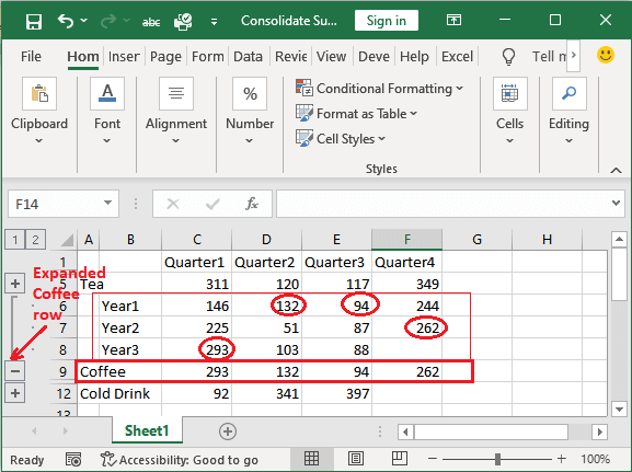

In the above screenshot, we have circled the maximum value in each column for the Coffee row (all three workbooks consolidated data).

You can understand this consolidated data with the help of the below table.

Result: After calculated consolidate summery

Firstly, all years values placed in same order with the help of label and then maximum value is found as resultant from it for each product.