| |

Excel Top/Bottom RulesAre you bored of looking at large data worksheets (containing numbers and text) again and again? Microsoft Excel provides quick help to present large chunks of data in an easily readable format. Many of you might have guessed it, and indeed you are true; it's the powerful Conditional formatting tool that enables Excel users to apply customized formatting to cells that satisfy specific criteria. Top/Bottom Rules is another cool feature of the Conditional Formatting tool in MS Excel that enables you to apply specific formatting to your worksheet cells that satisfy a statistical condition. This feature is often used as color-based formatting to emphasize, highlight, or distinguish among large data. It allows identifying different cell values with a glimpse. What is Excel Top/Bottom Rules?"The Conditional Formatting TOP/Bottom Rules in Excel allows the user to highlight the cell that satisfies the criteria (Top 10 items..., Bottom 10 items..., Top 10%..., Bottom 10%..., Above Average... or Below Average...) in the selected range." Top/Bottom Rules is a part of Conditional Formatting that enables you to apply formatting to cells that satisfy a statistical condition in the range.(for example, below average, within top 10 items, or below 10%, etc.). NOTE: The specified criteria will only be applied to Excel cells containing numeric data.The Excel Top/Bottom Rules option is listed in the Conditional Formatting menu, found in the 'Styles' group of the Home tab on the Excel ribbon. As soon you select this option, a secondary window pops up displaying the various sub-category options of Top/Bottom Rules. 
Top/Bottom Rules Options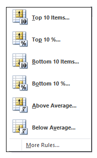
When we select the Top/Bottom Rules from the Conditional Formatting menu, the Top Bottom secondary window appears (refer to the below image). Excel Top/Bottom Conditional Formatting further offers 6 different built-in options to easily highlight the cell(s) which has the highest or lowest values from the range of selected cells. This enables the users to choose the formatting to apply to cells meeting the desired criteria.
Top/Bottom Appearance Options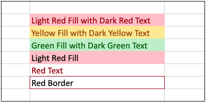
Microsoft Excel offers the pre-defined appearance options for conditionally formatting and highlighting the cells. The various options are as follows:
Example 1 - Excel Conditional Formatting Top/Bottom Rules for Top 10 items.The below-given table represents the total achieved sales target of each employee in one year. We will apply conditional formatting to classify the TOP 10 highest sales amount with the given data.
Solution: Below given are the detailed steps to find the Top 10 values in our Excel worksheet using the inbuilt Top/Bottom rules option: STEP-1 Select the range of cells Select the entire range of cells or the array, in which you wish to highlight the top10 values using the top/bottom rule conditional formatting. In our case, we have selected the cells from B3 to C16. Refer to the below image: 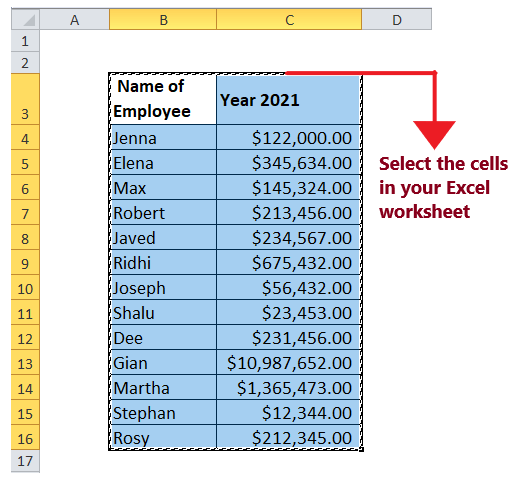
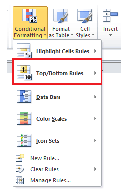
Step 2: Click on Conditional Formatting Top/Bottom Rules
Step-3 Click on TOP 10 Items Once you complete the above steps, a secondary window will pop up on your screen showing all the Top/Bottom Rules since we are asked to select only the top 10 sales figures in the question. So we will select the TOP 10 Items?' Refer to the below image: 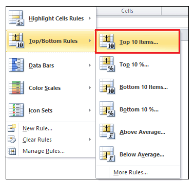
STEP 4: Fill the Data entries As soon as you select Top 10 items, another window will appear (refer to the below image) asking you to fill entries to format cells that rank in the top: 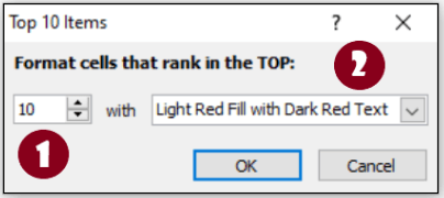
1. In the first field we will mention the numbers and by using the tiny arrow we will change the number of items to top 10. Note: The default Top/Bottom Percent is 10, though the user can specify any whole number up to 100.2. In the second field, we will select the color options to format and highlight the top 10 cells. Here, we have selected the Light Red Fill with Dark Red Text appearance option. Note: You can customize the formatting color according to your requirement. Just click on the custom format option from the appearance dropdown. Another window will appear through which you can change the font style, border, and highlight the top 10 cells with customized color.Step-4 The top 10 cells will be highlighted As a result you will notice all the top 10 sales cells are filled with pink color and the text is highlighted with red color. Look out at the below figure for the resulting output. 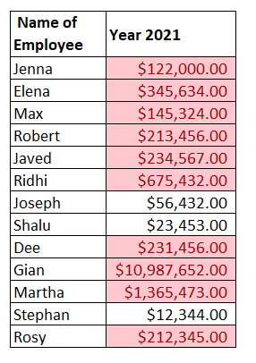
Eureka! Now you have learned how to apply a conditional formatting rule for the Top 10 items in your excel worksheet. Similarly following the above steps you can find the bottom 10 values. Example 2 - Excel Conditional Formatting Top/Bottom Rules with bottom 10 items.We will apply conditional formatting to highlight the Bottom 10 lowest sales figure with the given data.
Below given are the detailed steps to find the Bottom 10 values in our Excel worksheet using the inbuilt Top/Bottom rules option: STEP-1 Select the range of cells Select the entire range of cells or the array, in which you wish to highlight the bottom values using the top/bottom rule conditional formatting. In our case, we have selected the cells from B3 to C16. Refer to the below image:
Step 2: Click on Conditional Formatting Top/Bottom Rules
Refer to the below image: 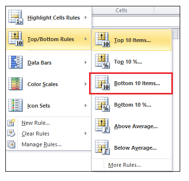
STEP 4: Fill the Data entries As soon as you select Bottom 10 items, another window will appear (refer to the below image) asking you to fill entries to format cells that rank in the BOTTOM: 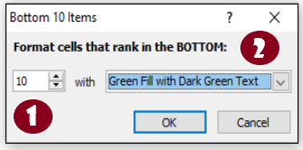
1. In the first field we will mention the numbers and by using the tiny arrow we will change the number of items to Bottom 10. Note: The default Top/Bottom Percent is 10, though the user can specify any whole number up to 100.2. In the second field, we will select the color options to format and highlight the bottom 10 cells. Here, we have selected the Green Fill with Dark Green Text appearance option. Step-4 The bottom 10 cells will be highlighted As a result you will notice all the bottom 10 sales figure cells are filled with green color and the text is highlighted with dark green color. Look out at the below figure for the resulting output. 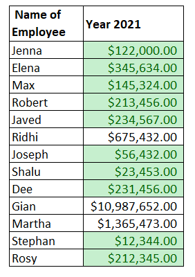
Done! The bottom 10 values are highlighted in different colors. Example 3 - Excel Conditional Formatting Top/Bottom Rules with Top 10% and bottom 10%.We will apply conditional formatting to highlight the top 10% values and bottom 10% values with the given data.
Below given are the detailed steps to find the Top 10% values and Bottom 10% values in our Excel worksheet using the inbuilt Top/Bottom rules option: STEP-1 Select the range of cells Select the entire range of cells or the array, in which you wish to highlight the top 10% values using the top/bottom rule conditional formatting. In our case, we have selected the cells from B3 to C16. Refer to the below image:
Step 2: Click on Conditional Formatting Top/Bottom Rules
Refer to the below image: 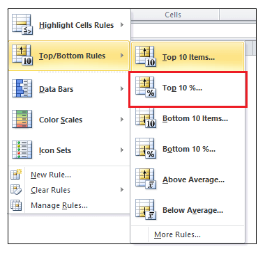
STEP 4: Fill the Data entries As soon as you select Top 10%..., another window will appear (refer to the below image) asking you to fill entries to format cells that rank in the top: 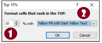
1. In the first field we will mention the numbers and by using the tiny arrow we will change the number of items to top 10. Note: The default Top/Bottom Percent is 10, though the user can specify any whole number up to 100.2. In the second field, we will select the color options to format and highlight the top 10% cells. Here, we have selected the Yellow Fill with Dark Yellow Text appearance option. Step-4 Cells values with Top 10% value will be highlighted As a result you will notice that the 10% cells are filled with yellow colour and the text is highlighted with dark yellow colour. Look out at the below figure for the resulting output. 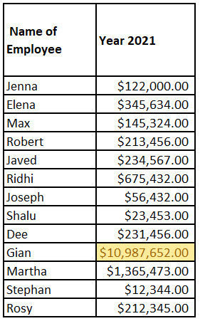
Step 5: Repeat the above steps with the Bottom 10% Repeat the same steps, but instead choose Bottom 10%... from the conditional formatting window. 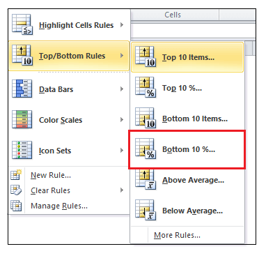
Select the "Light Red Fill" appearance option. As a result you will notice, the fastest values are also highlighted with Red colour: 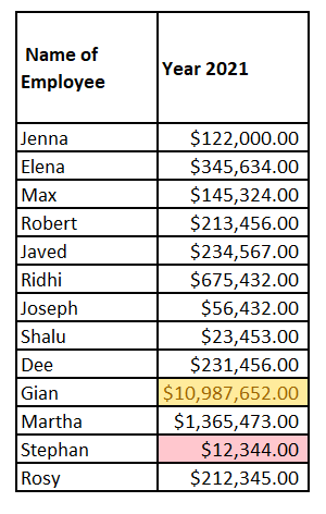
Example 4 - Excel Conditional Formatting Top/Bottom Rules with Above Average and Below Average.We will apply conditional formatting to highlight the above average and below average sales amount with the given data.
Below given are the detailed steps to find the above average values and below average values in our Excel worksheet using the inbuilt Top/Bottom rules option: STEP-1 Select the range of cells Select the entire range of cells or the array, in which you wish to highlight the below average values using the top/bottom rule conditional formatting. In our case, we have selected the cells from B3 to C16. Refer to the below image:
Step 2: Click on Conditional Formatting Top/Bottom Rules
Refer to the below image: 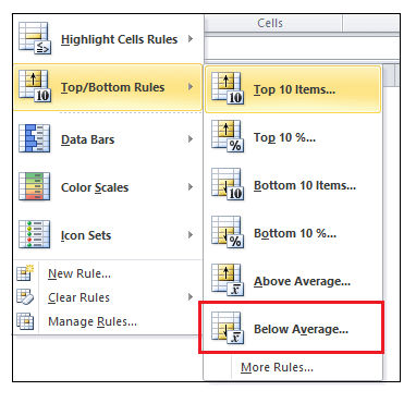
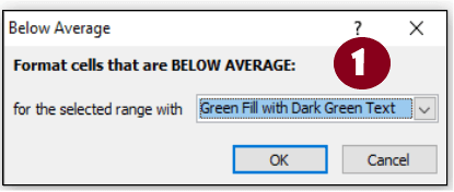
STEP 4: Fill the Data entries As soon as you select Below Average, another window will appear (refer to the below image) asking you to appearance drop box to format cells:
Step-4 The cells consisting above average cell values will be highlighted As a result, you will notice all the above-average cells are filled with Green color, and the text is highlighted with dark green color. Note: To ensure we have calculated the average and you cross-check whether the highlighted values are above this average value or not.Look out at the below figure for the resulting output. 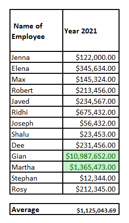
Step 5: Repeat the above steps with Below Average Repeat the same steps, but instead choose Below Average... from the conditional formatting window. 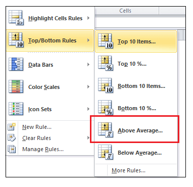
Select the "Light Red Fill" appearance option. As a result you will notice, the above average cell values are also highlighted with Red colour: 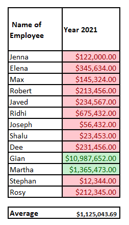
Next TopicCopy Worksheet in Excel
|
 For Videos Join Our Youtube Channel: Join Now
Feedback
- Send your Feedback to [email protected]
Help Others, Please Share


