| |

Microsoft ExcelMicrosoft Excel is an office use application designed by Microsoft. It comes with the Office Suite with several other Microsoft applications, like as Word, PowerPoint, Access, Outlook, and OneNote, etc. It is supported in Windows as well as Mac operating system too. Moreover, the Microsoft Excel is one of the most suitable spreadsheet programs that help us to store and represent the data in tabular form, manage and manipulate data, create optically logical charts, and more. Excel provides us the worksheet to create a new document in it. We can save the Excel file with .xls extension. What is Formula?In Microsoft Excel, the formula is used to define the relationship between the given variables as well. Generally, the formula involves symbols and various mathematical operators like as addition, subtraction, multiplication, and division. Formulas are used in enormous fields like science, education, research, finance, and various developing as well as developed fields. The purpose of the formula is to just find out the required solution to the problem, and based on the requirement, the formula is modified respectively. Why make use of the formula for finding solutions?There are several reasons why the formula is important for the calculations:
Formulas in Microsoft ExcelBy default, Microsoft Excel primarily provides various formulas to calculate the data. The reasons why formulas are used in Microsoft Excel are as follows:
How to enter formulas in Excel?Now to type a formula in Microsoft Excel, the following steps need to be followed as well: Step 1: First of all we are required to select a new cell, namely B1, to enter the formula as well. Step 2: Now after that, we need to enter the formula in the cell which is preceded by the equal to sign (=) respectively. 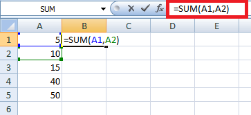
Step 3: And by just pressing the enter button, the result will be displayed in the selected cell as well. 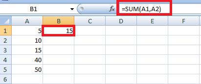
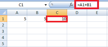
Excel FormulasMicrosoft Excel usually contains a wide range of formulas for each mathematical operation. The formulas primarily return the required result for the data and the result even though contains an Error respectively. And the variety of Microsoft Excel formulas is listed as follows: AdditionThe addition is considered as one of the most important arithmetic operations that can be used to sum or count the given values. The symbol for the addition is plus (+) sign. Moreover, the various formulas that are used for the addition in Microsoft Excel are as follows: 1. By making use of the '+' operator By making use of the '+' operator, the values that are present in the worksheet are added in Microsoft Excel .
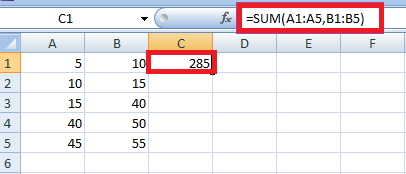
SUM FunctionAnd now the SUM function in Microsoft Excel is used to sum or count the specified cell or cell range respectively. The formula would be =SUM (A1, B1) to count the data in the specified cell. And to count the data for the specified range, the formula would be =SUM (A1:A5). 1.1 Sum function with multiple ranges In this, if the requirement is to just add out the multiple data ranges, the formula would be modified as =SUM (A1:A5, B1:B5, C1:C5). Here A1:A5, B1:B5, and C1:C5 are cell ranges.
2. 2 Sum function with Conditions If the requirement is to just add the given data that are based upon the conditions, the SUM function is modified which are based on the conditions respectively.
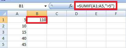
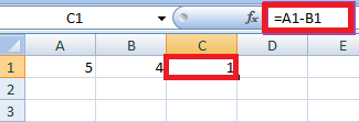
Similarly, the syntax will get varied for the conditions like lesser than, not equal to, equal to, etc. SubtractionSubtraction is considered one of the other most important arithmetic operations that can be used to find out the difference between the given values and it is the inverse of addition. The symbol for subtraction is plus (-) sign. 1. By making use of the '-' operator By making use of the '-' operator, the values which are present in the worksheet are subtracted in the Microsoft Excel Sheet.
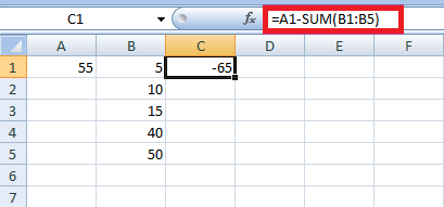
2. Sum function for Negative Values The Sum function is used to subtract out the range of values that are present in the given cell as well.
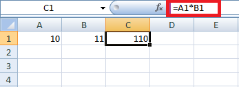
MultiplicationMultiplication is termed to be the other most important type of arithmetic operations that multiply two numbers to get out the product. The term involved in multiplication is multiplicand and multiplier as well. The symbol represents multiplication, Asterisk (*) Dot (.) Multiply symbol (x) 1. By making use of the asterisk Symbol The asterisk symbol in Microsoft Excel is used to multiply the given values, and the symbol is represented by the (*) sign effectively.
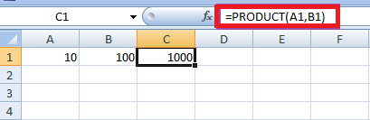
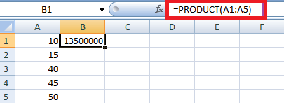
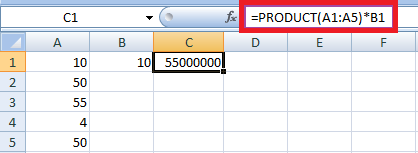
2. By making use of the Product Function As the name implies, the Product function is used to multiply two given values.
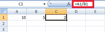
DivisionThe division is one of the other important arithmetic operations which divide the specified value into equal parts, and it is the inverse of multiplication. The symbol denotes it, Horizontal fraction bar (/). Division symbol (÷). 1. By making use of the '/' operator The '/' operator is primarily used to divide out the specified values.
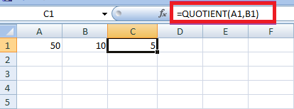
2. By making use of the Quotient Function The quotient function returns the quotient of the dividing values which is an integer.
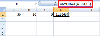
AverageThe average function is purposely used to find out the mean of the given numbers, and the average function is calculated by dividing the total value by the total Count of numbers in the data. The formula that is used to calculate the Average Function in Microsoft Excel is as follows: =AVERAGE (A1, B1, and C1). Here A1, B1, and C1 are the name of the cell.
CountThe Count function counts the number of data present in the specified range.
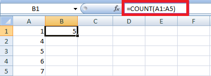
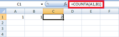
The COUNT function counts the cells which contain only the numerical values. 1. COUNTAIf the data contains a mixture of the text as well as the alphabet, the COUNTA function counts all the cells containing the data. It does not count the blank cells. The syntax used is none other than: =COUNTA (A1, B1)
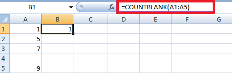
2. Countblank () The count blank () function in Microsoft Excel is used to count out the blank cell in the data, and if in case the data contains a mixture of the blank cells, then the count blank () function displays the number of the blank cells in the given data as well. The syntax used is, =COUNTBLANK (range) Here A1:A5 is called the cell range.
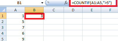
3. Count if () And the Count if () is an in-built function in Microsoft Excel that is used to count out the cells in the given range which are based upon certain conditions or criteria as well. The syntax for Count if the () condition is: =COUNTIF (range, criteria) In which,
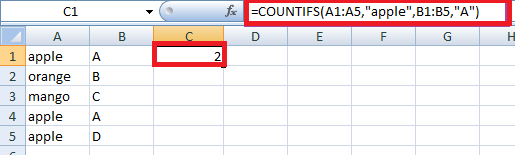
4. Counties The Countif function counts the range of the cells which are based upon the multiple criteria. The syntax for the Countif function is: =COUNTIFS (range1, critera1, range 2, criteria 2,..) In which,
And the Countifs function can accept around 127 range or criteria respectively.
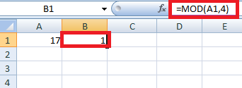
MODULUSNow the Modulus function in Microsoft Excel is used to return out the remainder of the dividing values, and the terms which are involved in the division are divisor and dividend as well. The MOD represents the Modulus function. The syntax to perform the Modulus function is as follows, =MOD (A1, B1) Here A1 and B1 is the cell name. And in the formula either the dividend is specified directly or by cell name.
Here A1 is the divisor, and the value 4 is the dividend. And both the divisors, as well as the dividend, are entered directly in the formula as, =MOD (25, 4). 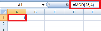
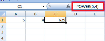
PowerThe power function in Excel raises the given number to the specified power value as well, and the formula that can be used to find out the power of the given value in Excel is as follows: =POWER (A1, B1) Here A1, B1 is called the cell value.
And the power value is entered directly or referred to in the cell name. To directly enter the power, the syntax will be: =POWER (A1, 5). The formula A1 contains the value raised to the power of 5. 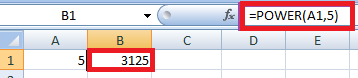
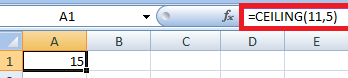
CEILINGThe ceiling function in Microsoft Excel is primarily used to round a number to the nearest multiple of the specified number, and the syntax of the Ceiling function is none other than the: =CEILING (number, significance). The number usually defines the value rounded, and significance is the multiple to which we want to round as well.
The CEILING function rounds the number, so if it is already the multiple of the significance, it returns the number without any change. CEILING (10, 5) returns 10, as 10 is already a multiple of 5. 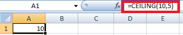
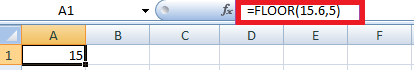
FLOORThe FLOOR function works opposite to the CEILING function. It rounds a number down to the nearest multiple of the specified number, and the syntax of the FLOOR is, =FLOOR (number, significance) The number primarily defines the value which is rounded, and significance is the multiple to which we want to round respectively.
The FLOOR function usually rounds the number, so if it is already the multiple of the significance, it returns the number without any change as well.
FLOOR (15, 5) returns 15, as 15 is already a multiple of 5 respectively. 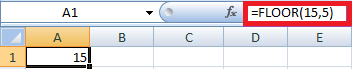
CONCATENATEConcatenation is joining or the combining of two or more strings or characters.
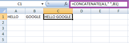
Another, Syntax for CONCATENATE function is none other than the =CONCATENATE (A1&" "&B1) 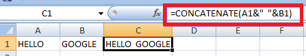
LENAs the name suggests the particular LEN function returns the total length of the characters in the given specified cell, and it counts the special characters as well as the spaces respectively.
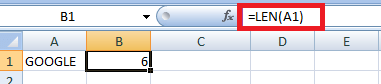
The LEN function displays the result as six, and the Count of the total characters in cell A1 respectively. REPLACEAs the name implies that the REPLACE function which replaces the specified text string with another one. The syntax for the REPLACE function will be like this: =REPLACE (old_text, start_num,num_chars,new_text) Here start_num refers to the characters' index position that needs to be replaced. num_chars defines the number of characters that need to be replaced as well.
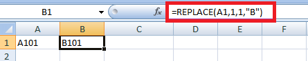
Next, if cell A1 contains the name Vijay which needs to be replaced with Ajay, then the formula will be written as =REPLACE (A1, 1, 2, "A"). 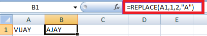
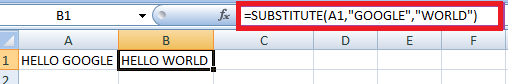
SUBSTITUTEAnd the SUBSTITUTE function replaces the existing text with the given new text. The syntax for the SUBSTITUTE function is as follows, =SUBSTITUTE (text, old_text, new_text,[instance_num])
Besides all this, the [instance_num] refers to the index position of the present text more than once as well. And if the cell contains text strings that are repeated more than once, the position of the text wants to be mentioned in the given formula as well.
=SUBSTITUTE (A1, 2007, 2023, 2) And the output will be displayed as follows, "MS EXCEL 2007, MS Word 2023" The second position of 2007 is replaced with 2023. In the example of substituting both the year with the same year, then the formula will be written as: =SUBSTITUTE (A1, 2007, 2023) The result will be "MS EXCEL 2023, MS Word 2023". 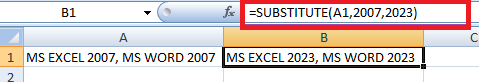
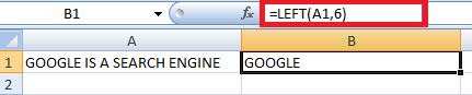
LEFT, RIGHT, MIDLEFT FunctionNow the LEFT function in Microsoft Excel usually returns the text which is left of the starting position of the given specified text as well.
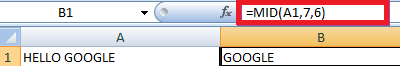
MID FunctionThe MID function in Microsoft Excel is purposely used to extract the specific text from the cell. The syntax of the MID function is as: =MID (text,start_num,num_chars) In the formula, The text primarily indicates the specified text in the cell where the particular text is extracted. Start_num usually represents the starting position of the specified text as well. Num_chars represents the number of characters extracted from the specified text.
Right FunctionThe Right function in Microsoft Excel extracts the specified number of characters from the right side of the text string as well. The syntax is as follows: =RIGHT (text,[num_chars]) The text represents the cell where the specified characters are extracted. In which the Num_chars represents the number of the characters that need to be extracted as well. This argument is an optional one, and if this argument is not mentioned, then the RIGHT function extracts one of the characters from the right of the string respectively.
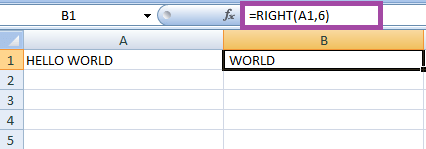
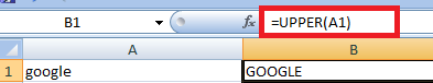
Here the RIGHT function displays the result as World respectively. Upper, Lower, and Proper CaseUpperAs the name indicates, the Upper function converts all the specified text into Upper Case. And the syntax for the function is, =UPPER (text)
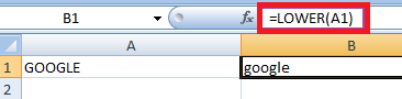
LowerNow the Lower function in Microsoft Excel is used to convert all the specified text into Lower Case as well. The syntax for the function is, =LOWER (text)
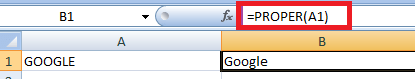
Proper CaseIt was well known that, the respective proper case function in Microsoft Excel is used to convert the first letter of the specified text into a capital letter and the remaining text into lowercase as well. The syntax of the proper case, =PROPER (text)
NOW ()And the NOW () function displays the system's current date as well as the time. The syntax for the NOW () function is, =NOW () Enter the syntax in any of the cells and just after that press the "Enter" Button as well. The current date and time of the system will be displayed respectively. 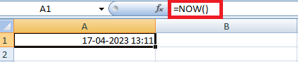
TODAY ()And the TODAY () function in Microsoft Excel is used to display the system's current date. The syntax for the TODAY () function is, =TODAY () Now we need to enter the syntax in any of the cells and just after that, we need to press the "Enter" button. The current date of the system will be displayed as well. 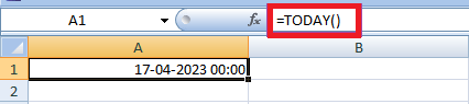
DAY ()The DAY () function primarily returns the day of the Month. A month comprises the day from 1 to 31. 1 denotes the first day of the Month, while 31 denotes the last day of the month.
=DAY (TODAY ()) In any of the cells, the result will be today's date respectively. 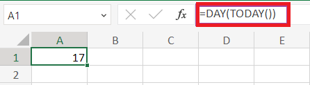
MONTH ()As the name implies that the MONTH () function is used to return the Month of the year. The Month comprises 1 to 12, 1 in January, and 12 in December.
=MONTH (TODAY ()) In any of the cells, the result will be the current Month. 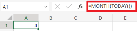
YEAR ()As the name implies, the YEAR () function returns the Year from the date value effectively.
=YEAR (TODAY ()) in any of the cells, and the result will be the current year, 2023. 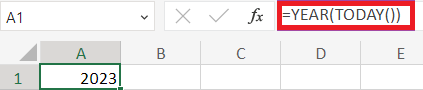
TIME ()The TIME () function in Microsoft Excel is used to convert the specified hours, minutes, and seconds into time format, which are entered as Excel Serial Number.
The result will be displayed at 8:40 P.M respectively. 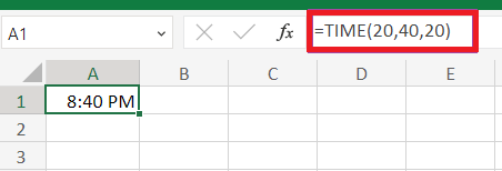
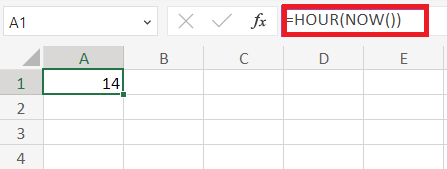
HOUR, MINUTE, SECONDThe Hour function primarily displays the hour value from the current time starting from 0 to 23, and here 0 indicates 12 AM, and 23 indicates 11 PM.
Minute ()The Minute () function is used to return the minute from a time value where the number ranges from 0 to 59. For example: To display the current minute, we need to enter the syntax in the new cell as =MINUTE (NOW ()), and just after that we need to press the "Enter" Button and the Minute Function will return the current minute of the hour. 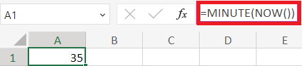
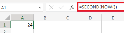
Second ()The Second () function in Microsoft Excel is used to return the second from a time value where the number ranges from 0 to 59 respectively.
Dated if ()The Dated if the () function returns out the difference between two dates in terms of the years, days, or months.
And if we want to calculate the age of a person, we need to enter the syntax as =DATEDIF (A2, B 2, "y") and just after that we need to press the "ENTER" Button. The result will be displayed as 2, which is a person's age. 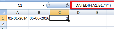
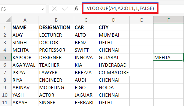
VLOOKUP ()As the name implies, the VLOOUP () function is called the "Vertical Lookup" and looks for the specified data that are present in the table's leftmost column. It returns the value present in the specified row as well as the column. The syntax for the VLOOKUP function is, =VLOOKUP(lookup_value, table_array,col_index_num,[range_lookup])
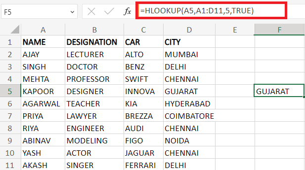
HLOOKUPAs the name implies, HLOOKUP stands for Horizontal Lookup, which looks at the value in the top row of a table. It displays the value in the same column from a row that the user specifies. The syntax for the HLOOKUP function is as follows: =HLOOKUP(lookup_value,table_array,row_index_num,[range_lookup])
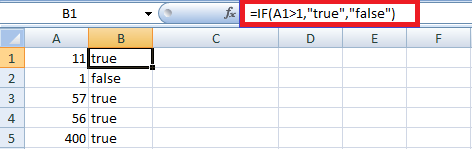
IF FunctionThe IF is a logical function that will return the particular value if the given condition is TRUE, and if the given condition is FALSE, and then it will return another value. The syntax for the IF function is: =IF(logical_test, [value_if_true], [value_if_false])
IF ERRORThe IF ERROR is one of the normal functions in Microsoft Excel, where it handles Errors in the formula. If the formula contains an error, it returns an expression or a value of the expression. The syntax of the IFERROR is: =IFERROR (value, value_if_error)
The value_if_error is optional. If this option is not included in the formula, it returns a default error message. If it is included, it displays a message about what the user has entered in the formula. 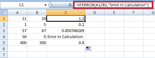
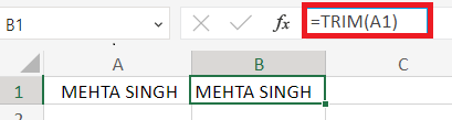
TRIMAs the name suggests, the TRIM function removes the extra space in the cell. It removes the space from the start and end of the text, whereas it doesn't remove the space between the texts respectively. The syntax for the TRIM function is, =TRIM (text)
MAX and MINThe MAX function in Microsoft Excel is used to find the maximum number in the given range. The syntax for the MAX function, =MAX (number1, [number 2],...) Either the number or ranges can be entered in the formula. 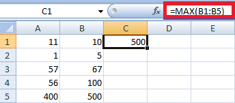
The MIN function usually finds out the minimum number in the given range as well. The syntax for the MIN function, =MIN (number1, [number 2],...) 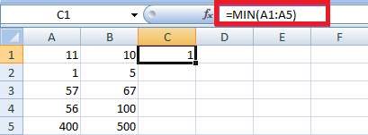
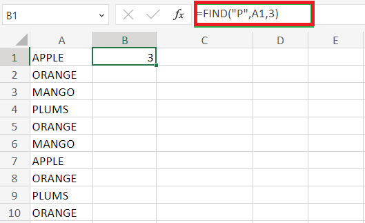
FINDThe FIND function finds out the position of the specified text string which is present inside another text string, and it will return the position of the text string if the formula is correct, or it returns the #VALUE Error. The syntax for the FIND formula, =FIND (find_text, within_text,[start_num])
SumproductThe Sumproduct function multiplies out the elements in the ranges or arrays, will add the products, and returns the result in a single element as well. The syntax for the Sumproduct is: =SUMPRODUCT (array 1,[array 2],[array 3]) 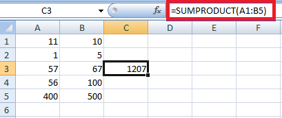
UniqueThe unique function is used to return the unique values that are present in the list. Values include text, alphabet, time, date, etc. The syntax for the unique function is: =UNIQUE (array,[by_col],[exactly_once]) 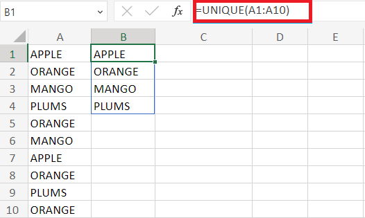
SortThe Sort function in Microsoft Excel is used to return the selected data in ascending or descending order. The syntax for the Sort function is: =SORT (array, [sort_index], [sort_order], [by_col]) 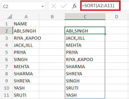
ISODD and ISEVENThe ISODD function returns the result as TRUE if the value is ODD otherwise it will return the result as FALSE if the value is EVEN. It returns the #VALUE error if the given value is not numeric respectively. The syntax for the ISODD function: =ISODD (value) 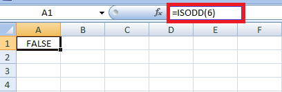
And the ISEVEN function returns the result as TRUE if the value is EVEN. It returns the result as FALSE if the value is ODD, otherwise, it will be returning the #VALUE error if the given value is not numeric as well. The syntax for the ISEVEN function: =ISEVEN (value) 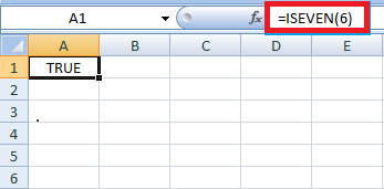
TEXT BEFOREThe TEXTBEFORE function in Microsoft Excel is used to return the text which occurs before the given data. And the syntax for the TEXTBEFORE function is: =TEXTBEFORE (text, delimiter, [instance_num], [match_mode], [match_end], [if_not_found]) 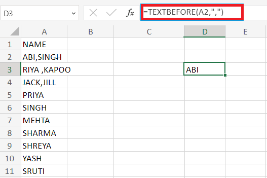
EXACT and MATCHThe match function returns the position of the lookup value where it is present in a row, column, or table respectively. The syntax for the MATCH function is: =MATCH (lookup_value, lookup_array, [match_type]) 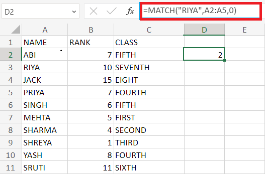
As the name suggests that the EXACT function usually returns the result as TRUE if the compared string is exactly matched, and it will return the result as FALSE if the compared string is not matched. The exact function is case-sensitive as well. The syntax for the EXACT function is: =EXACT (text 1, text 2) 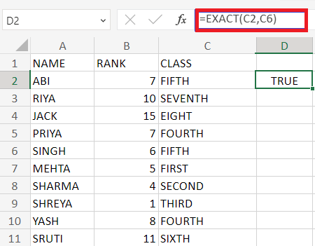
REPT functionThe REPT function repeats the given character a specified number of times. The syntax for the REPT function is: =REPT (text, number times) 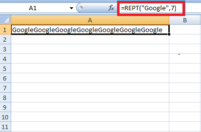
TransposeThe transpose function primarily changes the orientation of the given array or the range in the given table. If the given range is horizontal, then the range is converted to vertical. And if in case the given range is vertical, then it will be get converted to a horizontal range as well. Syntax of the transpose function is: =TRANSPOSE (array) 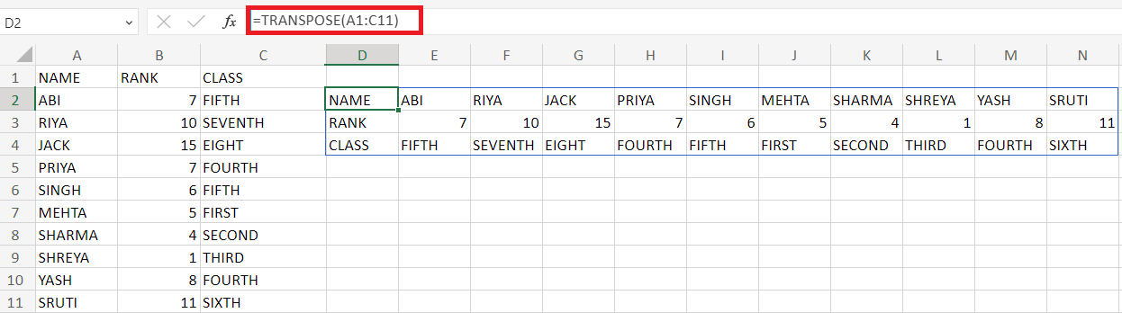
IS NUMBERThe ISNUMBER in Microsoft Excel returns the result as TRUE if a cell contains the number and it will return the FALSE if not. The syntax for the ISNUMBER is, =ISNUMBER (value) 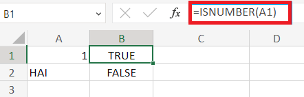
DropThe drop function usually returns the subset of the array in the specified rows as well as the columns. The number of rows and the number of columns that need to be removed in the given data is mentioned in the given formula.The syntax of the Drop function is: =DROP (array,[rows],[col]) 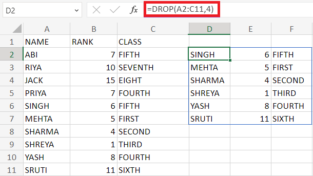
ABS functionThe ABS function is termed the "absolute function" which returns the absolute value of the given data respectively. It returns a positive number if the specified value is a negative number. And the syntax for the ABS function is: =ABS (number) 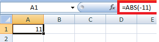
SummaryThe formula usually plays an important role in the calculation, and in this tutorial, some of the formulas are listed, that are used in Microsoft Excel for calculating the data. By default, it contains enormous formulas based on the data. |
 For Videos Join Our Youtube Channel: Join Now
Feedback
- Send your Feedback to [email protected]
Help Others, Please Share


