Setting Colors in Excel

MS Excel or Microsoft Excel is feature-rich spreadsheet software that enables users to record values within cells and adjust formatting accordingly using various built-in tools. When adjusting the appearance of an Excel sheet, colors play an important role. There are many elements in an excel sheet where the colors can be changed as per the choice. However, the most common fields include the background color of the cells and the font color of the values entered within the cells.

This article discusses the different ways to change or set colors in Excel. The article discusses common ways to set colors for the fonts and backgrounds of cells. Also, there are some specific methods for changing the color based on certain conditions.

General Methods of Setting Colors in Excel

The general methods include using built-in tools present on the Excel ribbon. We can easily change or switch the cell's background or the text/ value colors using these tools.

Setting Background Color for selected Cell (s)

When we create a new sheet in Excel, we see that all the cells are white. White is the default background color of all Excel cells. However, it is not limited to just white. Instead, we can replace it by either choosing the desired color from the existing standard colors or creating custom colors for each respective cell in Excel.

To set the desired color for the background of one or more selected cells, we need to perform the following basic steps:

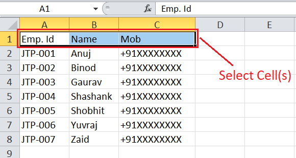
• First, we need to select/ highlight the cells to color. To select non-contiguous cells, we must click on each cell while holding the Ctrl key.
  
• After selecting the desired Excel cells, we need to go to the Home tab and click the drop-down arrow next to the Fill Color option under the Font group, as shown below:
  
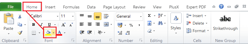
  Besides, we can use the shortcut "Alt + H, H" without quotes to quickly access the Fill Color tool.
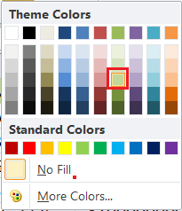
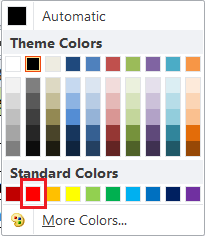
• In the next window, Excel displays various themes colors and the standard colors that we can choose to apply to the selected cells.
  
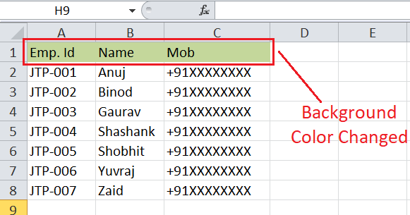
• We must click on any of the desired colors, and the same will be immediately inserted into the selected cells as the background color.
  
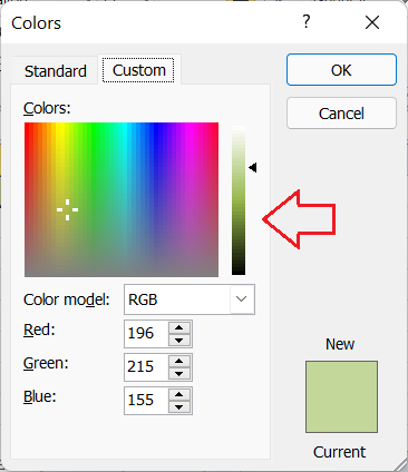
  Despite this, if we don't like the color or don't see the color we want, we can access More Colors and choose any custom color from the Colors dialogue box.
  

It is also possible to use a different background color in the entire worksheets by changing the background color of all the cells. We can use the 'Ctrl + A' shortcut to select all the cells in a worksheet. But this can hide the gridlines. We can use cell borders around all colored cells to improve worksheet readability in such a case.

Setting Foreground Color (font color) for selected Cell (s)

By default, the foreground color or the color used in values within the Excel cells is black. Like the cell background, we can also change or replace the colors of the values present in Excel cells.

To set the desired color for the foreground of one or more selected cells, we need to perform the following basic steps:

• First, we need to select/ highlight the desired cells to change the colors of fonts. When selecting non-contiguous cells, we can click on each cell while holding the Ctrl key.
  
• Next, we need to navigate the Home tab and click the drop-down arrow next to the Font Color option under the Font group, as shown in the following image:
  
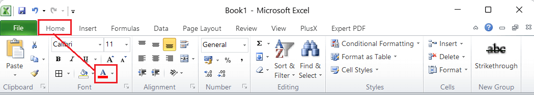
  To quickly access the Font Color tool on the ribbon, we can use the "Alt + H + FC" shortcut without quotes.
• We will get the multiple color options under the themes colors and the standard colors category in the next window.
  
  We can click on any desired color to apply it to values within the selected cells.
  
  We can select the 'More Color' option to choose/create a custom color for the foreground.

It is recommended not to use the same foreground color as the background color of the cell because otherwise, the text or values will not be displayed or become invisible.

Note: Instead of changing fonts and background color of excel cells using the color tool, we can also try themes in excel. Excel themes enable us to quickly change the text fonts, colors, or appearance of many other worksheet elements throughout the workbook. To use the theme, we can go to Page Layout > Themes.

Conditional Methods of Setting Colors in Excel

It is also possible to set up certain conditions using the conditional formatting options and then change the colors accordingly in Excel. Using conditional formatting, the cells' background color and foreground colors can change based on the values within the cells.

Although there can be several conditions when we might want to change colors in Excel, the following are some common scenarios to change colors by cell value:

Setting Colors if Negative/Positive

Suppose we have the following excel sheet where the prices of some commodities have either increased or decreased compared to the original price. Changes in prices are also shown within the sheet, along with the price at which prices have increased (positive) or decreased (negative).

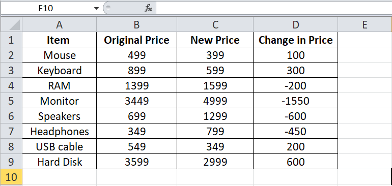
It will be hard to locate the specific cells with negative or positive values when we have a large data set. Therefore, it is better to highlight a specific cell color, font color, or both.

When we want to change the color based on whether the cell values are negative or positive, we need to perform the following steps:

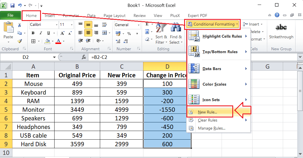
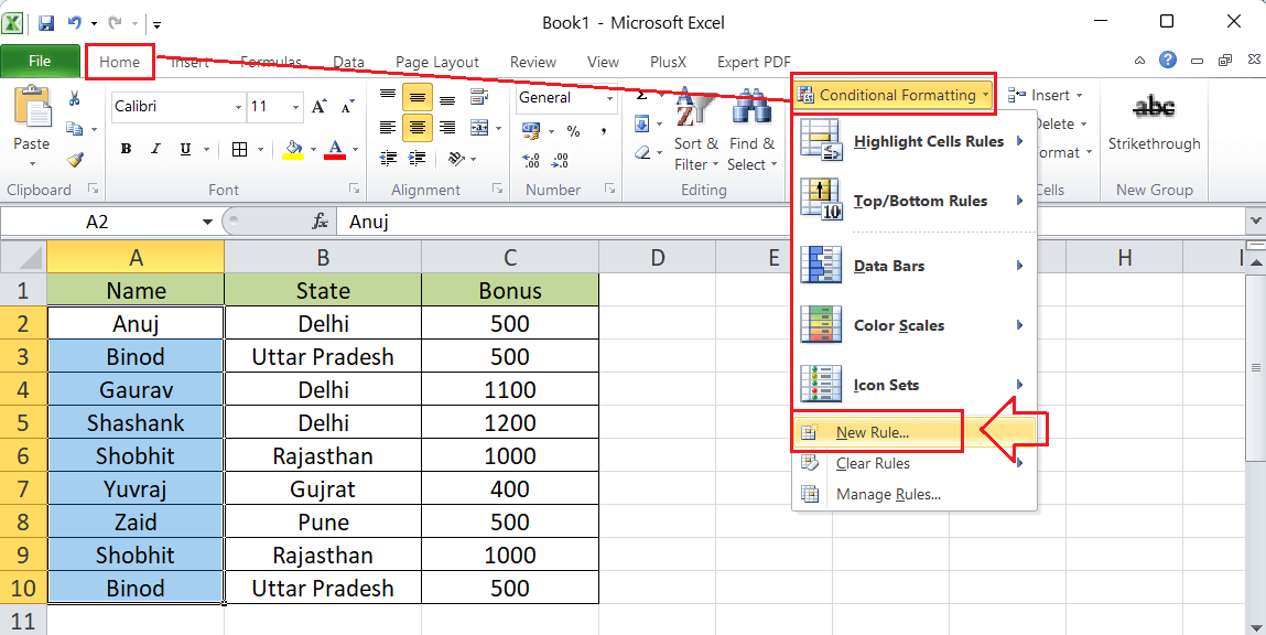
• First, we need to select the cell or a range (D2:D9, in our case) where we want to apply colors and then navigate to Home > Conditional Formatting > New Rule. Excel will launch the New Formatting Rule dialogue box.
  
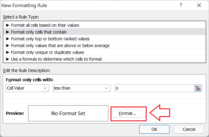
• We choose the 'Format only cells that contain' option under the 'Select a Rule Type' category in the dialogue box. Then, under the 'Edit the Rule Description', we must select the 'Cell Value' option from the first box, the 'less than' option in the second box, and enter zero (0) in the last box. It will look like this:
  
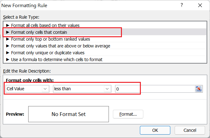
  In this way, we modify the rule to select all the negative values from the selected range. When we want to highlight the color of positive values, we can choose the 'greater than' option from the second/ middlebox.
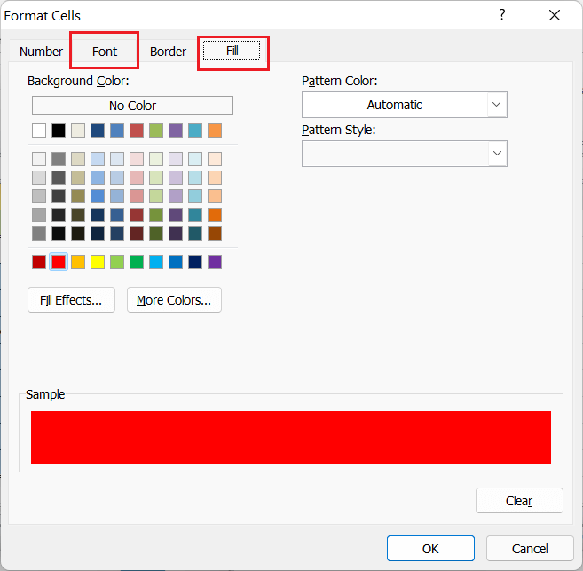
• After setting up the rules, we need to go to the Format Cells window to configure desired colors for background and/or fonts. Therefore, we must click the 'Format' button from the 'New Formatting Rule' dialogue box, as shown below:
  
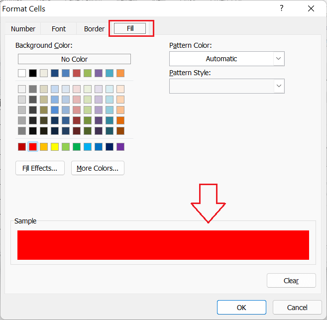
• After clicking the Format button, we will see the 'Format Cells' dialogue box. We need to click on the Fill tab and choose the desired color that we want to set up for the background of cells.
  
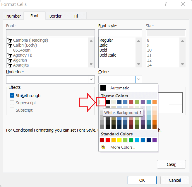
  Likewise, we can go to the Font tab and select one color we want to use as the font color for the applied rule.
  
• After choosing the desired colors, we must click OK > OK to close both dialogue boxes. After closing the Format Cells dialogue box, we can check the preview of colors in the 'New Formatting Rule' dialogue box, as shown below:
  
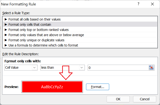
  The colors of negative values will instantly change, as shown below:
  

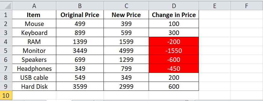
In this way, we can set up colors for negative/ positive values. The values will change in real-time. If the price change becomes positive from negative, the colors will also change accordingly. This particular method of setting colors is useful in the stock exchange prices chart.

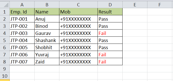
Setting Colors if duplicate values

Suppose we have the following excel sheet with the names of some employees who are expected to receive the bonus amount.

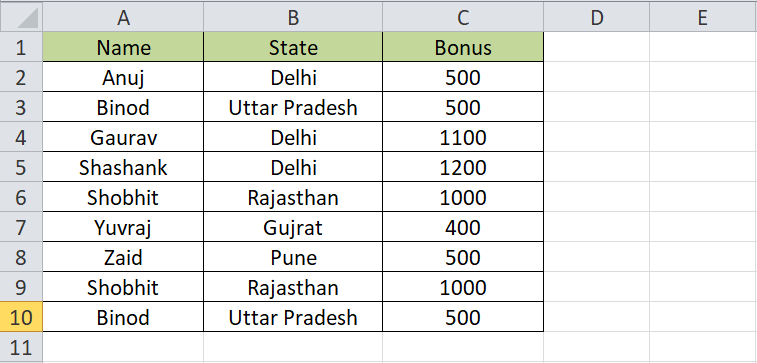
However, some repeated names are in the list, which is somewhat a mistake. It is difficult to find all such repeated or duplicate names if the list is long. Therefore, we can set a rule and a specific color on the duplicate values to find and fix them easily. For this, we need to do the following steps:

• First, we need to select the cells or a range (A2:A10, in our case) where we want to apply colors and then navigate to Home > Conditional Formatting > New Rule.
  
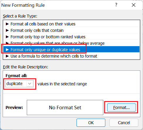
• In the New Formatting Rule dialogue box, we choose the 'Format only unique or duplicate values' option under the 'Select a Rule Type' category. Then, under the 'Edit the Rule Description', we must select the 'duplicate' option from the drop-down list. After that, we must click the Format button to configure color options.
  
• In the Format Cells dialogue box, we must go to the Fill and Font tab to choose the desired colors, respectively.
  
• After selecting the colors, we must click on the OK button from the Format Cells dialogue box and click OK again to close the New Formatting Rule dialogue box. All the cells with duplicate values will be colored as the specified color.
  

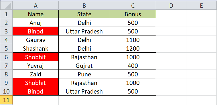
In the above image, the duplicate values are colored where the font color is white, and the cell's background color is red.

Setting Colors if blank

Excel enables users to apply certain rules with formulas using the conditional formatting feature. Using the formula, we can find the blank cells and configure the desired color for the respective cells.

Suppose we have the following excel sheet where students' attendance record (present or absent) is entered.

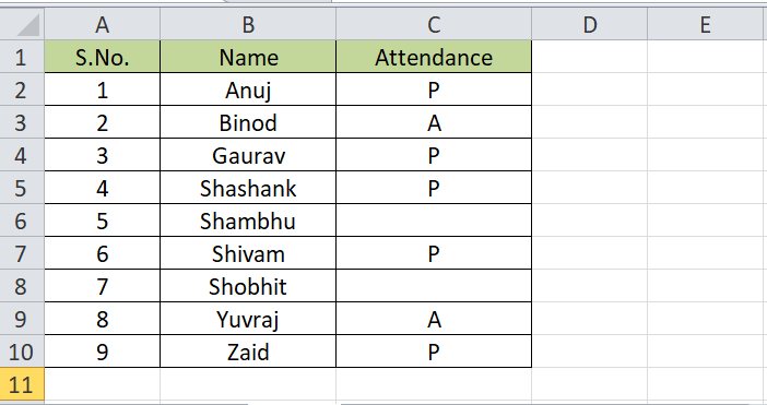
However, some students are not marked as present or absent, leaving the respective cells blank or empty. We can set a rule to detect and color these blank cells when the list is large. We need to do the following steps:

• First, we need to select the cells or a range (C2:C10, in our case) where we want to apply colors and then navigate to Home > Conditional Formatting > New Rule.
  
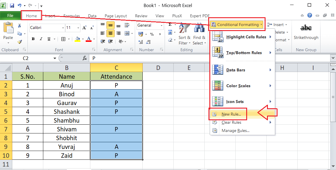
• In the New Formatting Rule dialogue box, we choose the 'Use a formula to determine which cells to format' option under the 'Select a Rule Type' category. Then, under the 'Edit the Rule Description', we must enter the formula '=IsBlank()' without quotes. After that, we must click or place the cursor between parenthesis and the supply the respective range, i.e., "=IsBlank(C2:C10)".
  
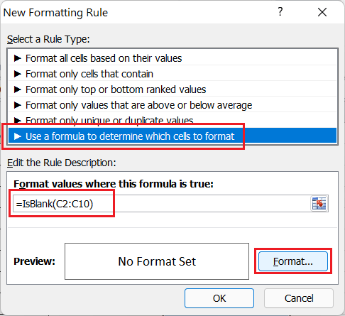
  In this way, we modify the formula to set up a rule to select all the blank cells from the selected range C2:C10.
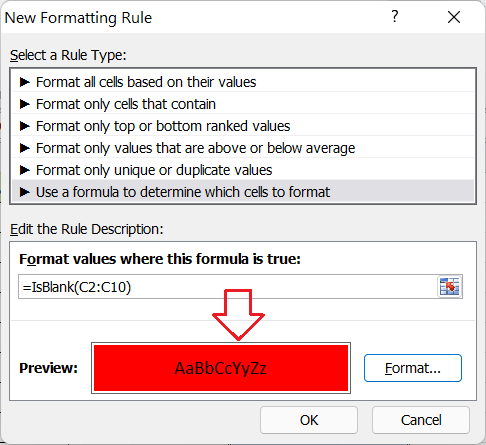
• Next, as discussed above, we should click on the Format button and select the desired color for the font and cell background.
  
• Lastly, we must click OK > OK to close dialogue boxes and apply the specified color on blank cells within the selected range.
  

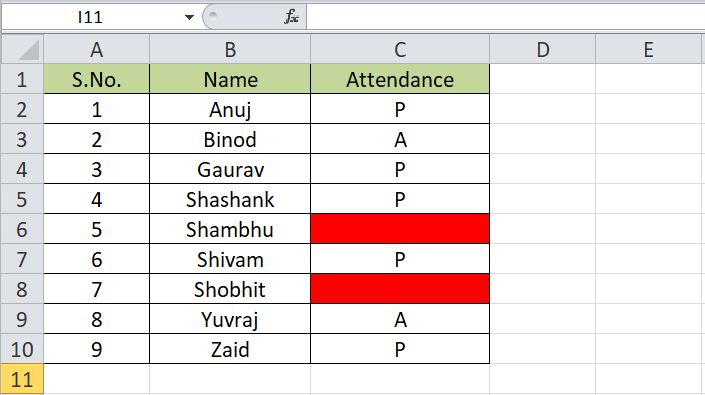
In the above image, blank cells are colored where the cell's background color is red. It is important to note that we must choose a specific background color for blank cells because choosing a font color does not make sense for blank cells.

Setting Colors if contain

When we need to change the cell background colors and/or foreground based on if certain values are present, we can easily set a rule accordingly using conditional formatting.

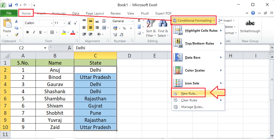
Suppose we have the following Excel sheet with employees' names and state-wise locations.

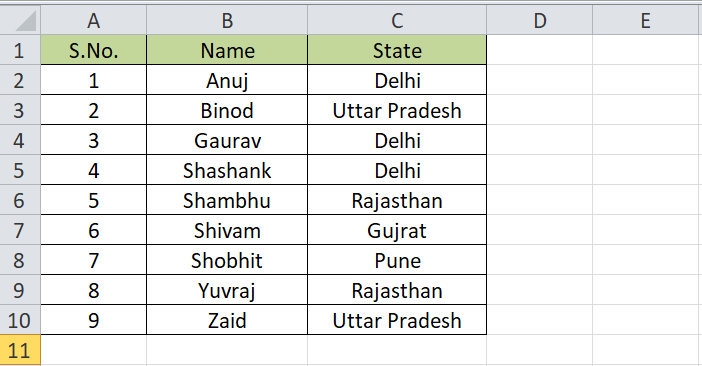
If we want to detect all employees who belong to Delhi, we can set a rule to detect cells with specific texts (Delhi, in our case) and choose the desired color for background and foreground accordingly. We need to perform the following steps to choose colors if cells have specific values:

• First, we must select the cells or a range (C2:C10, in our case) to apply colors and go to Home > Conditional Formatting > New Rule.
  
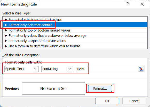
• In the New Formatting Rule dialogue box, we choose the 'Format only cells that contain' option under the 'Select a Rule Type' category. Then, under the 'Edit the Rule Description', we must select the 'Specific Text' option from the first box, the 'containing' option in the second box, and enter Delhi in the last box. It will look like this:
  
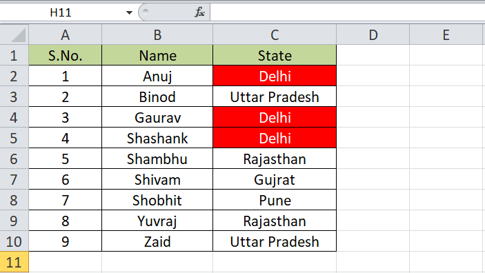
• Next, we must go to the Format Cells dialogue box and choose the desired colors for the background and foreground of the corresponding cells. Lastly, we need to click OK > OK.
  

Setting Colors based on Ranges (multiple conditions)

Suppose we have the following excel sheet in which the total marks of some students are in percentage.

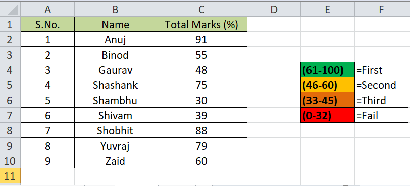
In our example sheet, we want to color or highlight specific cells based on the range of scores. For example, scores of 33-45 would be orange, 46-60 would be yellow, 61-100 would be green, and everything else (0-32) would be red. In this case, we have to create multiple rules based on ranges of values for selected cells. We need to follow the below steps to achieve this:

• First, we must select the cells or a range (C2:C10, in our case) to apply colors and go to Home > Conditional Formatting > Manage Rules.
  
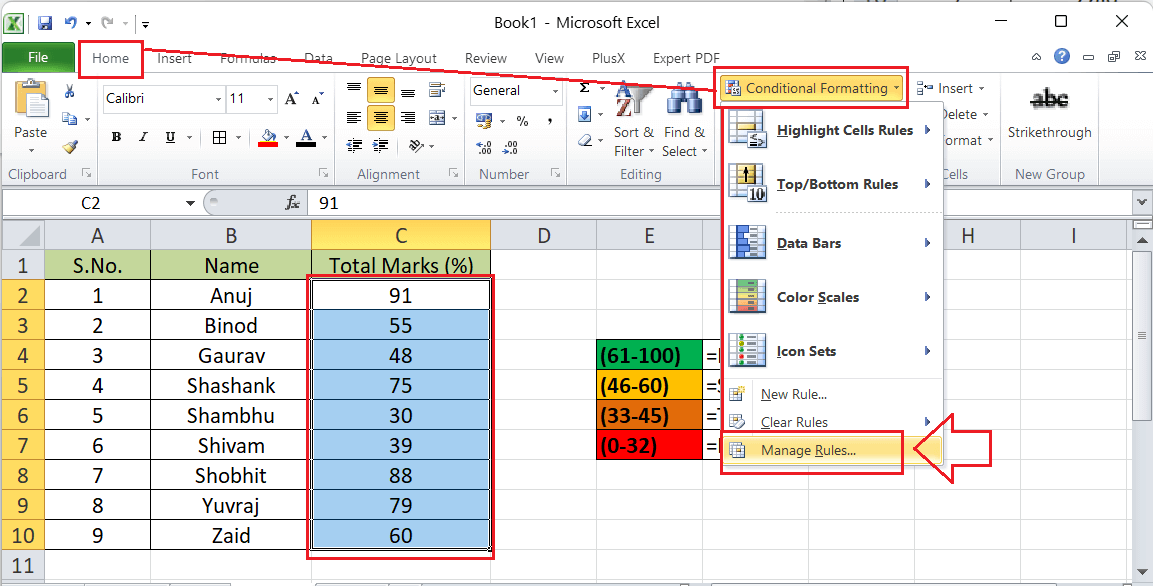
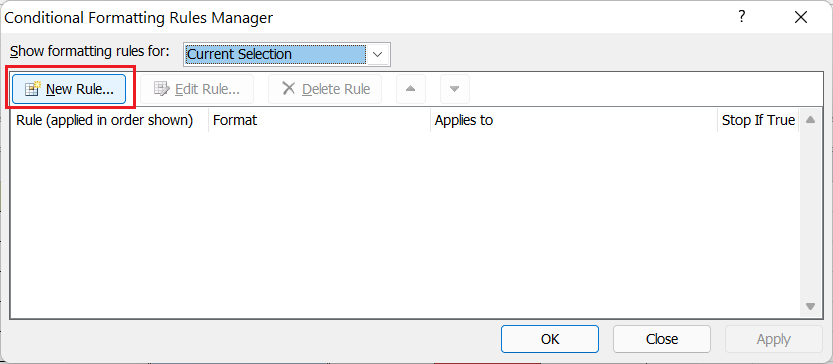
• Next, we must click the New Rule button from the Conditional Formatting Rules Manager, as shown below:
  
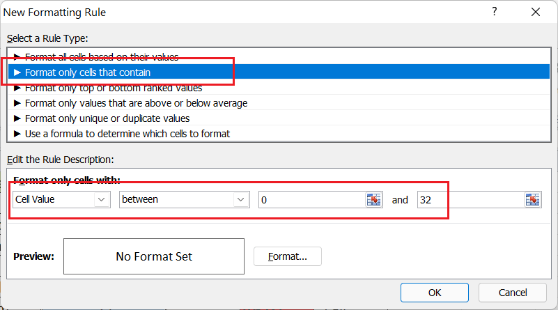
• In the New Formatting Rule dialogue box, we choose the 'Format only cells that contain' option under the 'Select a Rule Type' category. Then, under the 'Edit the Rule Description', we must select the 'Cell Value' option from the first box, 'between' option in the second box, and enter the minimum and maximum range of scores for the first condition (i.e., 0-32) in the following two boxes. It will look like this:
  
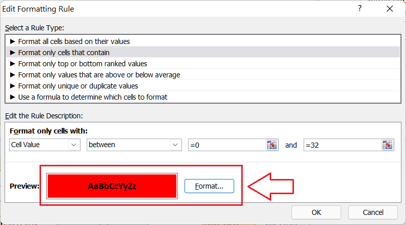
• After that, we must click the Format button and select the red color for the cell background, black color for the font and click OK to close the Format Cells dialogue box. The cells falling into the supplied range (0-32) will be colored by performing this step.
  
• Again, we must click the New Rule button from the Conditional Formatting Rules Manager. After that, we need to go through the above steps and set rules for other ranges of scores, such as 33-45, 46-60, and 61-100. Also, we must choose the colors for each range accordingly.
• Once all the rules and respective colors have been set up, we need to check all the applied rules for the selected cells from the Conditional Formatting Rules Manager. In our case, it looks like this:
  
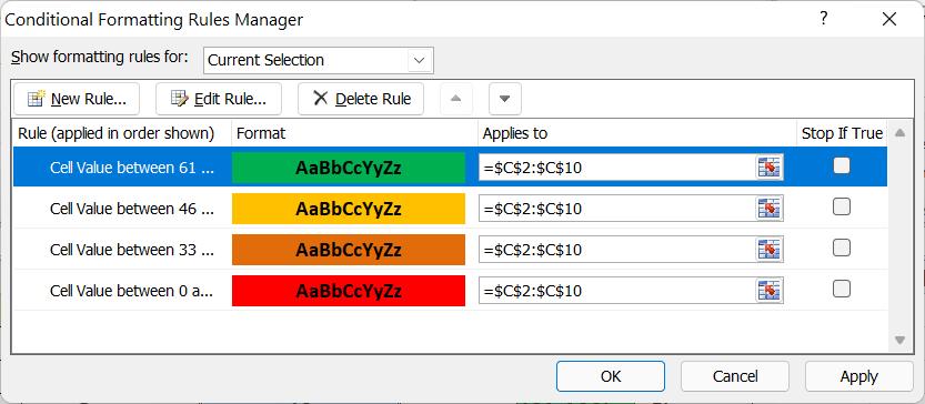
• Lastly, we must click the OK button from the Conditional Formatting Rules Manager to close the window. The selected cells will instantly be colored as per the applied rules and chosen colors.
  

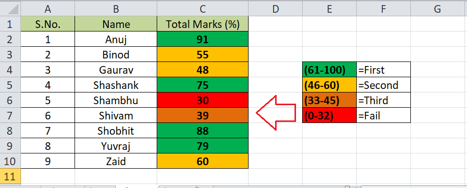
In this way, we can create rules based on specific ranges of values using multiple conditions and format the background and foreground colors accordingly.

Important Points to Remember

• Setting colors in Excel is also possible from the Format Cells dialogue box, which can be accessed using the shortcut "Ctrl + 1" without quotes after selecting the desired cell (s).
• Using too many colors or high-contrast colors can sometimes ruin the look of the entire worksheet.