Link State Routing

Link state routing is a technique in which each router shares the knowledge of its neighborhood with every other router in the internetwork.

The three keys to understand the Link State Routing algorithm:

• Knowledge about the neighborhood: Instead of sending its routing table, a router sends the information about its neighborhood only. A router broadcast its identities and cost of the directly attached links to other routers.
• Flooding: Each router sends the information to every other router on the internetwork except its neighbors. This process is known as Flooding. Every router that receives the packet sends the copies to all its neighbors. Finally, each and every router receives a copy of the same information.
• Information sharing: A router sends the information to every other router only when the change occurs in the information.

Link State Routing has two phases:

Reliable Flooding

• Initial state: Each node knows the cost of its neighbors.
• Final state: Each node knows the entire graph.

Route Calculation

Each node uses Dijkstra's algorithm on the graph to calculate the optimal routes to all nodes.

• The Link state routing algorithm is also known as Dijkstra's algorithm which is used to find the shortest path from one node to every other node in the network.
• The Dijkstra's algorithm is an iterative, and it has the property that after k^th iteration of the algorithm, the least cost paths are well known for k destination nodes.

Let's describe some notations:

• c( i , j): Link cost from node i to node j. If i and j nodes are not directly linked, then c(i , j) = ∞.
• D(v): It defines the cost of the path from source code to destination v that has the least cost currently.
• P(v): It defines the previous node (neighbor of v) along with current least cost path from source to v.
• N: It is the total number of nodes available in the network.

Algorithm

Initialization
N = {A}     // A is a root node.
for all nodes v
if v adjacent to A
then D(v) = c(A,v)
else D(v) = infinity
loop
find w not in N such that D(w) is a minimum.
Add w to N
Update D(v) for all v adjacent to w and not in N:
D(v) = min(D(v) , D(w) + c(w,v))
Until all nodes in N

In the above algorithm, an initialization step is followed by the loop. The number of times the loop is executed is equal to the total number of nodes available in the network.

Let's understand through an example: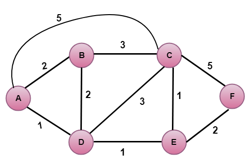

In the above figure, source vertex is A.

Step 1:

The first step is an initialization step. The currently known least cost path from A to its directly attached neighbors, B, C, D are 2,5,1 respectively. The cost from A to B is set to 2, from A to D is set to 1 and from A to C is set to 5. The cost from A to E and F are set to infinity as they are not directly linked to A.

Step 2:

In the above table, we observe that vertex D contains the least cost path in step 1. Therefore, it is added in N. Now, we need to determine a least-cost path through D vertex.

a) Calculating shortest path from A to B

b) Calculating shortest path from A to C

c) Calculating shortest path from A to E

Note: The vertex D has no direct link to vertex E. Therefore, the value of D(F) is infinity.

Step 3:

In the above table, we observe that both E and B have the least cost path in step 2. Let's consider the E vertex. Now, we determine the least cost path of remaining vertices through E.

a) Calculating the shortest path from A to B.

b) Calculating the shortest path from A to C.

c) Calculating the shortest path from A to F.

Step 4:

In the above table, we observe that B vertex has the least cost path in step 3. Therefore, it is added in N. Now, we determine the least cost path of remaining vertices through B.

a) Calculating the shortest path from A to C.

b) Calculating the shortest path from A to F.

Step 5:

In the above table, we observe that C vertex has the least cost path in step 4. Therefore, it is added in N. Now, we determine the least cost path of remaining vertices through C.

a) Calculating the shortest path from A to F.

Final table:

Disadvantage:

Heavy traffic is created in Line state routing due to Flooding. Flooding can cause an infinite looping, this problem can be solved by using Time-to-leave field