Binary Decision Tree

A Binary Decision Tree is a decision taking diagram that follows the sequential order that starts from the root node and ends with the lead node. Here the leaf node represents the output we want to achieve through our decision. It is directly inspired by the binary tree. Since each node can have a maximum of two nodes in the binary tree, in the same way, at each step, we have one or two steps in which we will choose one.

It is a decision-making algorithm used in Machine Learning when we have a lot of data and we want to get the result after processing at each step.

Without appropriate constraints, a Decision Tree might expand until only one sample-or a very small number-is present at each node. Due to this circumstance, the model becomes overfit and loses its ability to accurately generalize. This issue can be avoided by using a consistent test set, cross-validation, and a maximum allowable depth. Class balancing is another crucial factor to consider. Decision Trees can produce inaccurate results when a class is dominant because they are reactive to unbalanced classes. One of the resampling techniques, or the class weight option, which is offered by the scikit-learn implementations, can be used to alleviate this issue. By avoiding bias, a dominating class can be penalized proportionately.

Let's suppose in a dataset, we have n data points, and each point has m features. Then the decision tree might look like this where t is the threshold value: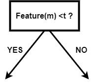

Single Splitting Node

So in the Binary Decision Tree, each node should be selected in such a way that the feature we choose for that node should be able to separate the data in the best way. If we choose such a node, it reduces the number of steps, and we get the target in less number of steps and complexity.

In real life, it is very difficult to select or find a feature that minimizes the structure of the Binary Decision Tree. The structure of the tree depends upon the feature we choose and the threshold value.

For example: We have a class of students where all the boys have black hair, and the girls have green hair. In the black color, there will be different lengths of the students, and in red, it will be different lengths. If our target is to get the composition of the data of black and green hair, then a simple binary decision tree can look like this: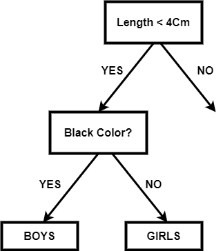

In the above tree, we have divided it based on the length of the hair and then divided it according to the hair color. Since we do not need the separation based on the length of the hair, so it is called impurity. Impurity nodes are added to the tree, which unnecessarily makes the structure bigger and more complex. If the impurity node is below the target node, then there is no problem.

So we can get the optimal tree of the above example like this: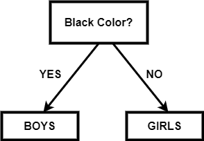

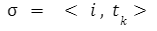
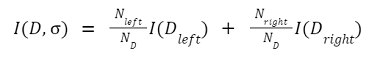
If we need the data about the hair length, then this node can be easily added below the leaf nodes.

Note: so, each node's selection can be represented in the below form:

In the above equation, we have two values where i represent the index of the dataset from which we want to split. In the root node, we will have a complete dataset so that i will be zero, and in successive steps, the dataset will be reduced. t_k represents the threshold value by which we split the dataset. So we have to be very careful while choosing the threshold because the threshold decides the structure of the tree. If our threshold is not good, then we can get a long tree to reach the target.

We can measure the total impurity, and our target would be to reduce the total impurity to reach the desirable node as soon as possible.

We can get the total impurity measure by the below formula:

Here D represents the complete dataset on which we are working. D_left and D_right represent the left and right node dataset which was created after splitting according to the threshold.

I represent the total impurity measure of the node.