Time Complexity of Kruskals Algorithm

We shall talk about Kruskal's algorithm in this post. We shall also examine the Kruskal's algorithm's difficulty, functionality, example, and implementation here.

However, we need first comprehend the fundamental concepts, such as spanning tree and least spanning tree, before going on to the technique.

An undirected edge-weighted graph's smallest spanning forest is found via Kruskal's method. Finding a minimal spanning tree is done if the graph is linked. (A minimal spanning tree is a collection of edges that forms a tree with every vertex in a linked graph where the weighted average of all the edges in the tree is minimized. A minimal spanning forest for a disconnected graph is made up of a minimum spanning tree for each linked component.) In graph theory, it is known as a greedy method since it continuously adds the next lowest-weight edge that won't cycle to the minimal spanning forest.

An undirected connected graph's spanning tree is a sub graph of that graph.

Minimum Spanning Tree - A minimum spanning tree is one in which the total edge weights are at their lowest value. The weight of the spanning tree is the total of the weights assigned to its edges.

Let's get to the major point now.

For a linked weighted graph, the least spanning tree is determined using Kruskal's Algorithm. The algorithm's primary goal is to identify the subset of edges that will allow us to pass through each graph vertex. Instead of concentrating on a global optimum, it adopts a greedy strategy that seeks the best outcome at each step.

How is the Kruskal algorithm implemented?

With Kruskal's method, we begin with the edges that have the lowest weight and keep adding edges until we get the desired result. The following are the steps to apply Kruskal's algorithm:

Sort all of the edges first from low weight to high weight.
Add the edge with the lightest weight to the spanning tree at this point. Reject the edge if it would otherwise result in a cycle.
Once we have included all of the edges, a minimal spanning tree will be produced.

The uses of Kruskal's algorithm include:

Wiring between cities may be laid out using Kruskal's method.
It is possible to utilize it to install LAN connections.

Kruskal's Algorithm Example

Let's now use an example to demonstrate how Kruskal's algorithm functions. An illustration will make it simpler to comprehend Kruskal's algorithm.

Let's say that a weighted graph is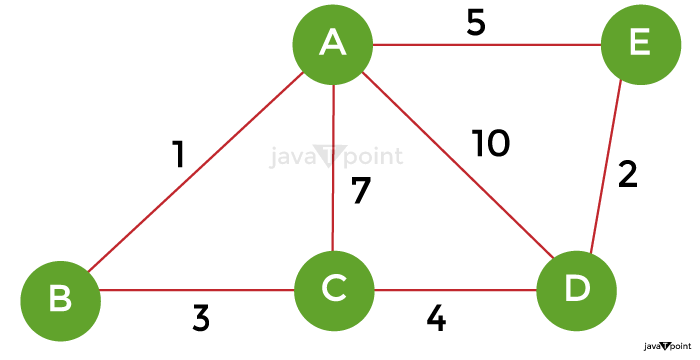

The table below provides the edge weights for the graph above.

Edge	AB	AC	AD	AE	BC	CD	DE
Weight	1	7	10	5	3	4	2

Sort the edges listed above now according to ascending weights.

Edge	AB	DE	BC	CD	AE	AC	AD
Weight	1	2	3	4	5	7	10

Let's start building the least spanning tree right now.

Step 1: Add the edge AB with weight 1 to the MST in step 1 first.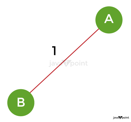

Step 2: Since the edge DE with weight 2 isn't producing the cycle, add it to the MST.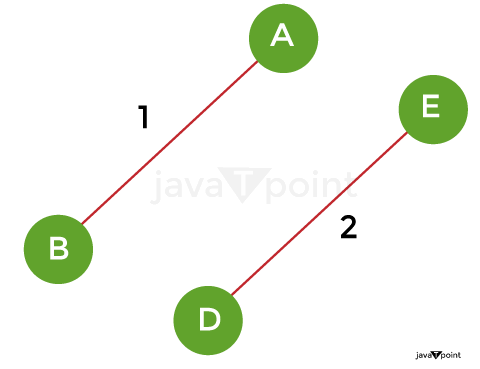

Step 3: Add the edge BC with weight 3 to the MST in step 3 because it does not produce a cycle or loop.

Step 4: Choose the edge CD with weight 4 to the MST at this point since the cycle is not being formed.

Step 5 - Next, choose weight 5 on the edge AE. This edge must be eliminated since including it would start the cycle.

Step 6: Pick the edge of the AC using weight in step 6." This edge must be eliminated since including it would start the cycle.

Step 7: Pick the edge AD with weight 10 in step 7. Throwing away this edge will prevent the cycle from starting.

Step 8: As a result, the final minimal spanning tree created using Kruskal's approach from the provided weighted graph is -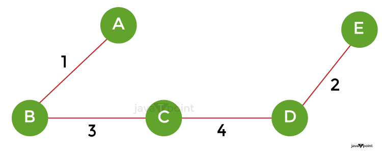

The cost of the MST is = AB + DE + BC + CD = 1 + 2 + 3 + 4 = 10.

In the above tree, the number of edges now matches the number of vertices minus 1. The algorithm so ends here.

Step 1: Create a forest F in such a way that every vertex of the graph is a separate tree.  
Step 2: Create a set E that contains all the edges of the graph.  
Step 3: Repeat Steps 4 and 5 while E is NOT EMPTY and F is not spanning  
Step 4: Remove an edge from E with minimum weight  
Step 5: IF the edge obtained in Step 4 connects two different trees, then add it to the forest F   
(for combining two trees into one tree).  
ELSE  
Discard the edge  
Step 6: END  

Time Complexity of Kruskal's Algorithm

The Kruskal method has an O(E logE) or O(V logV) time complexity, where E is the number of edges and V is the number of vertices.

A connected, undirected graph with all of its vertices is described as a spanning tree, which is a tree-like sub graph of the graph. Or, to put it in Layman's terms, it is a subset of the graph's edges that together form an acyclic tree, of which the graph's nodes are all members.

With the additional restriction of having the lowest weights among all conceivable spanning trees, the minimal spanning tree has all the characteristics of a spanning tree. Similar to spanning trees, a graph may have several potential MSTs.

Properties of a Spanning Tree

The following principles are held by a spanning tree:

The graph and spanning tree both have the same number of vertices (V).
The spanning tree has a fixed number of edges, which is one fewer than the total number of vertices (E = V-1).
There should only be one source of component, not more, so that the spanning tree is not disconnected.
There should be no cycles in the spanning tree, which means it should be acyclic.
The sum of the edge weights of all the spanning tree's edges is referred to as the overall cost (or weight) of the spanning tree.
There are several spanning trees that might be used for a graph.

Implementation of the Kruskal algorithm

Let's now examine how Kruskal's method was put into practice.

Create a C++ program that implements Kruskal's algorithm.

CODE:

// C++ program for the above approach
#include <bits/stdc++.h>
using namespace std;
// DSU data structure
// path compression + rank by union
class DSU {
	int* parent;
	int* rank;
public:
	DSU(int n)
	{
		parent = new int[n];
		rank = new int[n];
		for (int i = 0; i < n; i++) {
			parent[i] = -1;
			rank[i] = 1;
		}
	}
	// Find function
	int find(int i)
	{
		if (parent[i] == -1)
			return i;
		return parent[i] = find(parent[i]);
	}
	// Union function
	void unite(int x, int y)
	{
		int s1 = find(x);
		int s2 = find(y);

		if (s1 != s2) {
			if (rank[s1] < rank[s2]) {
				parent[s1] = s2;
			}
			else if (rank[s1] > rank[s2]) {
				parent[s2] = s1;
			}
			else {
				parent[s2] = s1;
				rank[s1] += 1;
			}
		}
	}
};

class Graph {
	vector<vector<int> > edgelist;
	int V;

public:
	Graph(int V) { this->V = V; }

	// Function to add edge in a graph
	void addEdge(int x, int y, int w)
	{
		edgelist.push_back({ w, x, y });
	}

	void kruskals_mst()
	{
		// Sort all edges
		sort(edgelist.begin(), edgelist.end());

		// Initialize the DSU
		DSU s(V);
		int ans = 0;
		cout << "Following are the edges in the "
				"constructed MST"
			<< endl;
		for (auto edge : edgelist) {
			int w = edge[0];
			int x = edge[1];
			int y = edge[2];

			// Take this edge in MST if it does
			// not forms a cycle
			if (s.find(x) != s.find(y)) {
				s.unite(x, y);
				ans += w;
				cout << x << " -- " << y << " == " << w
					<< endl;
			}
		}
		cout << "Minimum Cost Spanning Tree: " << ans;
	}
};

// Driver code
int main()
{
	Graph g(4);
	g.addEdge(0, 1, 10);
	g.addEdge(1, 3, 15);
	g.addEdge(2, 3, 4);
	g.addEdge(2, 0, 6);
	g.addEdge(0, 3, 5);
	// Function call
	g.kruskals_mst();
	return 0;
}

OUTPUT:

Following are the edges in the constructed MST
2 -- 3 == 4
0 -- 3 == 5
0 -- 1 == 10
Minimum Cost Spanning Tree: 19

Time Complexity: Either O (E*logE) or O (E*logV)

It takes O (E * logE) time to sort edges.
After sorting, the find-union method is used to iteratively traverse all edges. The maximum time for the find and union procedures is O (logV).
O (E * logE + E * logV) time is the measure of total complexity.
O (logV) and O (logE) are same since the value of E can only be at most O (V2) in size.
O (E* logE) or O (E*logV) is the general temporal complexity as a result.

Auxiliary Space: O (V + E), where V is the total number of edges in the graph and E is the total number of vertices.

Next TopicTravelling Salesman Problem

← prev next →