| |

Electricity Consumption Prediction Using Machine Learning
In today's fast-paced world, electricity consumption holds a vital position in fulfilling the energy needs of modern societies. As the demand for electricity keeps growing, optimizing energy usage becomes extremely important. Thankfully, advancements in technology have led to the emergence of machine learning, a potent tool that can predict electricity consumption with remarkable accuracy. Forecasting electricity consumption is a complex undertaking. It requires analyzing large volumes of historical data, such as past electricity usage, weather patterns, time of day, and seasonal changes. Although traditional methods offer some insights, they often struggle to capture intricate connections between these variables. Enter machine learning, a branch of artificial intelligence that equips computers with the ability to learn from data and make predictions without being explicitly programmed. Machine learning algorithms excel at discovering hidden patterns and correlations in vast datasets, making them a perfect fit for electricity consumption prediction. Advantages of Electricity Consumption Prediction Using Machine LearningElectricity consumption prediction using machine learning offers numerous advantages that can revolutionize the way we manage and optimize our energy resources. Some of the key advantages include:
Challenges of Electricity Consumption Prediction Using Machine LearningPredicting electricity consumption using machine learning comes with its fair share of challenges. While machine learning offers promising solutions, it is essential to be aware of the hurdles that may arise during the process. Some of the key challenges include:
About the DatasetThis dataset is a daily time series of electricity demand, generation, and prices in Spain from 2014 to 2018. It is gathered from ESIOS, a website managed by REE (Red Electrica Española), which is the Spanish TSO (Transmission System Operator) A TSO's main function is to operate the electrical system and to invest in new transmission (high voltage) infrastructure. (https://www.ree.es/en/about-us/business-activities/electricity-business-in-Spain) As a system operator, REE forecasts electricity demand and offers and runs daily actions. As a result of daily actions, a PBF Plan Básico de funcionamiento) is yielded. This is a basic scheduling of energy production (upon it, several mechanisms are triggered to ensure supply) Energy and prices data can be downloaded from: https://www.esios.ree.es/en OMIE (Operador del Mercado Iberico de Electricidad) is responsible for running those daily actions and also offers interesting data. ContentOriginal values are kept, so some names in Spanish are shown. The column name describes each time series, so I provide a description of each name:
Note: Original data format is maintained, just in case it is necessary to append new data downloaded from Esios. As a result, geo columns are null.Code:Importing LibrariesReading the DatasetOutput: 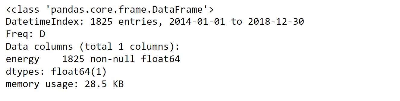
Output: 
Output: 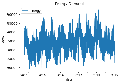
Output: 
We're in luck! There are no missing values in the dataset, and we have a four-year span of data to work with. Now, let's dive into the exciting part and calculate some date-related features to make our analysis go on. Output: 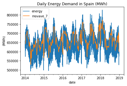
EDA(Exploratory Data Analysis)Analyzing the target variable involves studying its seasonality and trend. Our aim is to visually understand the patterns and fluctuations in the time series data without heavily relying on statistical techniques such as decomposition. By graphically examining the data, we can gain insights into the underlying patterns and trends that may exist. Target Analysis(Normality)Output: 
In terms of data distribution, negative skewness indicates that the data is not perfectly symmetrical and has a longer left tail. Additionally, the kurtosis value below 3 suggests that the tails of the distribution are slightly thinner compared to a normal distribution. This characteristic is known as platykurtic, indicating that the likelihood of encountering extreme values is lower than in a normal distribution. Output: 
Output: 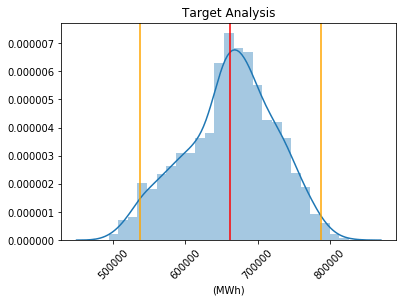
In general, the data does not exhibit a normal distribution as it displays a smaller left tail and a reduced likelihood of observing extreme values compared to normally distributed data. Output: 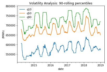
Output: 
Output: 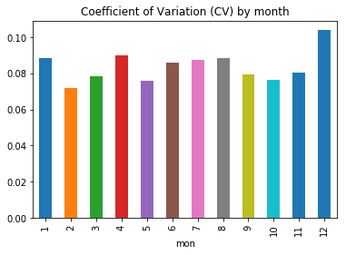
Output: 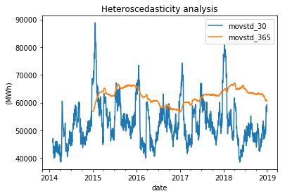
When considering shorter time periods such as quarters and months, volatility tends to vary, but over the long term (in a yearly window), it remains relatively stable. As a result, potential predictors need to account for the seasonal pattern in variance. Output: 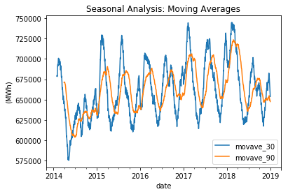
Output: 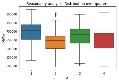
Output: 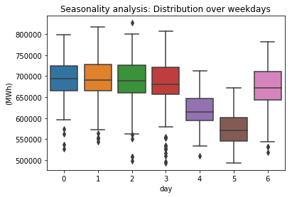
As anticipated, there are distinct seasonal patterns observed in the data when considering quarters and weekdays (with Monday represented as 0). Output: 
Output: 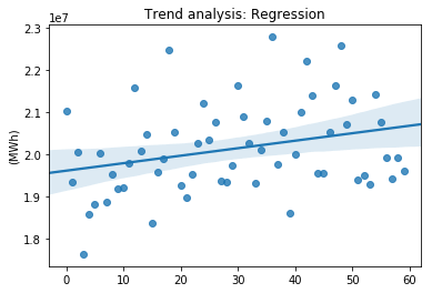
Output: 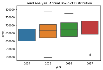
The energy demand shows a positive linear trend, or a slightly damped trend, which can be attributed to the steady economic growth resulting from the recovery from a previous recession. Feature EngineeringThe current challenge lies in developing automated features that can effectively handle seasonality, trend, and changes in volatility. These features should be able to adapt to the varying patterns and fluctuations observed in the data. Standardizing the data is a necessary step to enable the application of models that are sensitive to scale, such as neural networks or support vector machines (SVM). By standardizing the data, we ensure that the distribution shape remains unchanged while only altering the first and second moments, namely the mean and standard deviation. This process allows for more accurate and effective modeling of the data using these particular machine learning algorithms. Output: 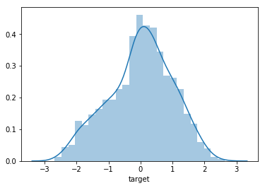
Output: 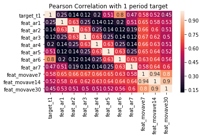
Output: 
Some features, such as AR_6 (AutoRegressive lag 6) and MOVAVE_7 (7-day moving average), exhibit a relatively strong linear correlation with the target variable. To validate this assumption and further investigate their predictive power, we will build various models and evaluate their performance using these features. By assessing the models' accuracy and predictive capabilities, we can determine the extent to which these features contribute to the overall predictive power of the models. Model BuildingIn this step, we have built two candidate models using a convenient feature in Scikit-Learn called MultiOutput Regression. This feature allows us to efficiently and automatically fit models that can predict multiple target variables simultaneously. By leveraging this framework, we can train our models to predict several target variables in a streamlined manner. This not only simplifies the modeling process but also enables us to evaluate the models' performance across multiple targets effectively. First, we will fit a baseline model using linear regression and compare it to a more advanced model, such as Random Forest. The linear regression model does not require extensive hyperparameter tuning and provides a solid foundation for our analysis. However, there are several considerations to keep in mind:
On the other hand, an advanced model such as Random Forest requires careful hyperparameter tuning to achieve optimal performance. Typically, this is done using techniques like GridSearch and Cross Validation (CV). However, using traditional CV methods with time series data poses challenges. This is because the data should not be shuffled as it follows a specific time structure. Fortunately, Scikit-Learn provides a helpful solution called TimeSeries Split. This technique allows us to perform GridSearch in a time-aware manner by preserving the temporal order of the data. It splits the data into sequential time-based folds, ensuring that each fold respects the chronological order of the observations. By using TimeSeries Split, we can iteratively train and evaluate our Random Forest model with different combinations of hyperparameters. This approach enables us to find the best set of hyperparameters that maximizes the model's performance on unseen future data points. Applying hyperparameter tuning in a time-aware manner is essential for time series data, as it ensures that our model's performance is more realistic and reliable. By leveraging the TimeSeries Split functionality in Scikit-Learn, we can effectively optimize our Random Forest model without violating the temporal structure of the data. Output: 
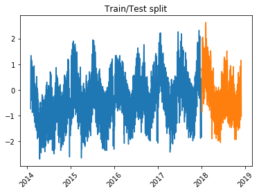
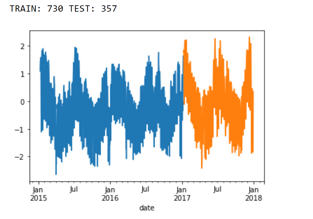
Splitting DataTo ensure an unbiased evaluation of our model's performance and conduct thorough residual analysis, we reserve the data points from the year 2018 as a separate holdout dataset. This means that we keep this data untouched during the model development process. Output: 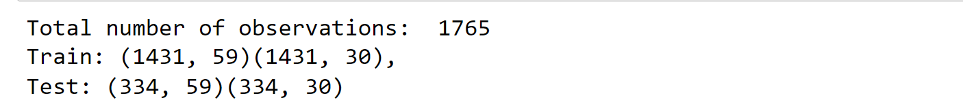
Baseline Model: Linear RegressionOutput: 
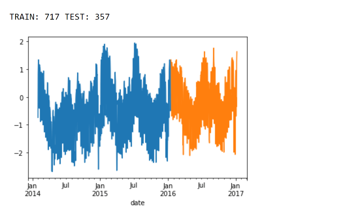
Train a Random Forest with Time Series Split to tune HyperparametersIn this particular example, we illustrate the use of the TimeSeriesSplit framework. With this approach, each fold of the data is constructed in such a way that the training data is closer to the beginning of the forecasting period. Output: 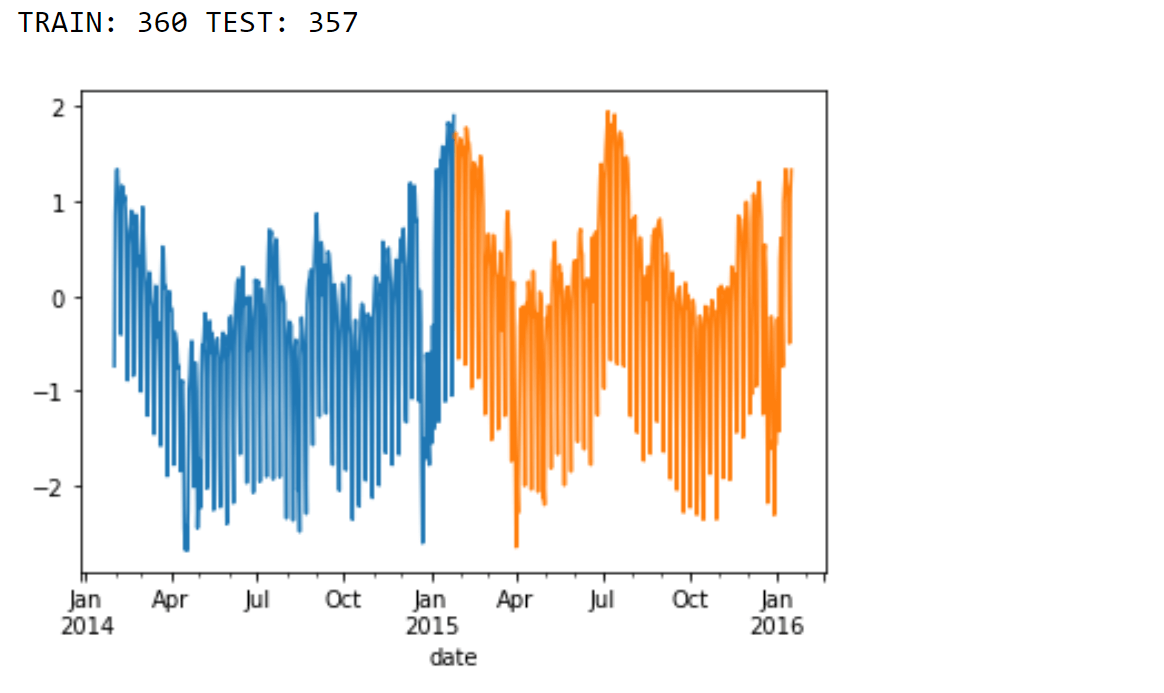
Output: 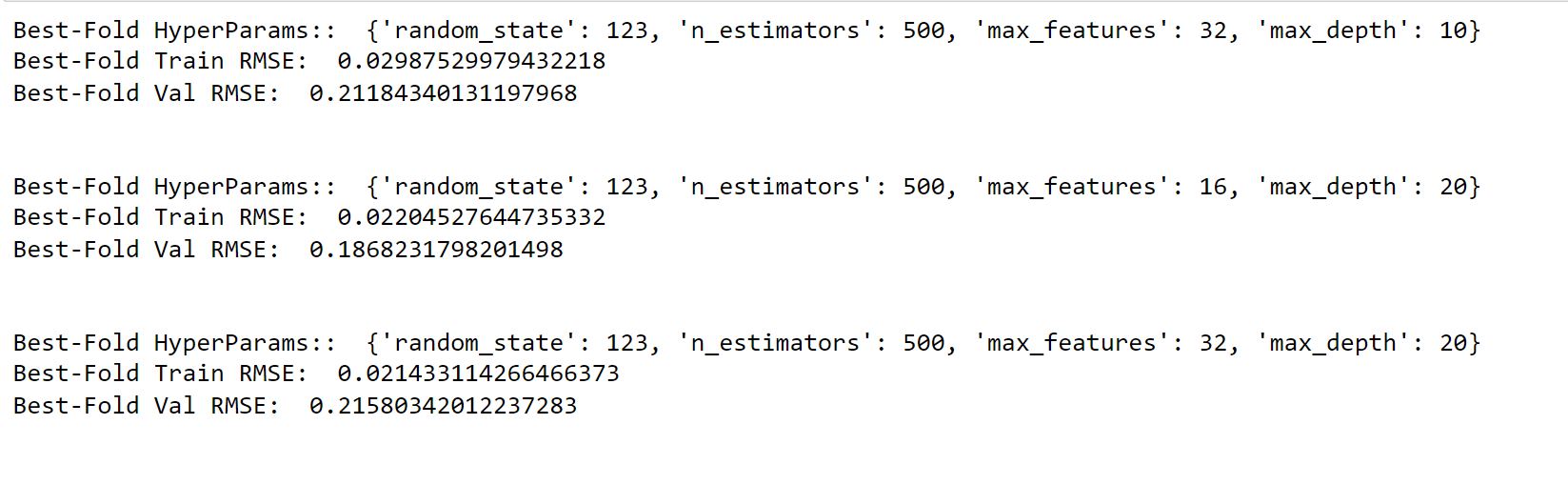
Utilizing Random Forest yields a significant enhancement in comparison to Linear Regression. However, it is essential to exercise caution as Random Forest models are constructed by bootstrapping the data, which may result in the loss of some time structure within the dataset. Feature ImportanceOutput: 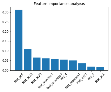
The results obtained from the model do not align with the findings of the correlation analysis, highlighting the influence of complex relationships and interactions on model performance. This aspect is crucial to consider, particularly when dealing with models such as ARIMA. Model AssessmentWhen evaluating the performance of the model, the Mean Absolute Percent Error (MAPE) is chosen as the performance metric instead of the commonly used Root Mean Square Error (RMSE). MAPE is considered more appropriate for this analysis as it is easier to interpret and communicate. The MAPE will be calculated using a one-period ahead model for the test period. Output: 
Output: 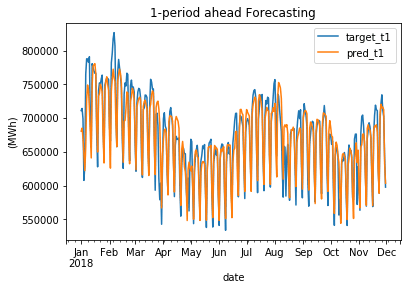
The MAPE value is slightly above 10%, which is quite remarkable considering the strong dependence of electricity demand on weather conditions. Moreover, it is important to note that February experienced exceptionally cold temperatures, making the result even more astonishing. Output: 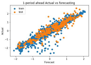
By plotting the actual values against the forecasted values, we can visually assess the model's ability to fit the training data and generalize it to the test data. Residual AnalysisOutput: 
Output: 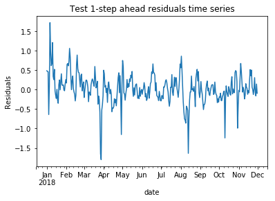
Output: 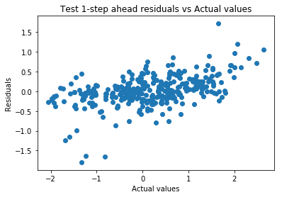
ForecastingMulti-period ahead model buildingOnce we determine the optimal set of hyperparameters, we can train a new instance of the Random Forest model using the most recent and relevant data. Typically, it is recommended to have at least two years of data to generate a long-term daily forecast. Let's proceed with retraining a collection of Random Forest models using the MultiOutput Regression feature. Lastly, it is important to evaluate the forecasting accuracy using the MAPE (Mean Absolute Percent Error) metric across multiple periods and determine if it remains consistent and stable. Output: 
Output: 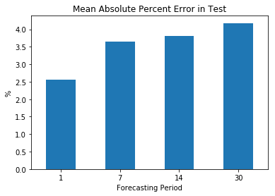
As expected, the forecasting accuracy improves when considering a shorter period. It is worth noting that having more data does not always guarantee better results. Additionally, the MAPE tends to increase as the forecasting horizon extends, but overall, it demonstrates a relatively stable pattern. Actual VS ForecastedAs mentioned before, a convenient method to evaluate the model's fit is by plotting the actual values against the forecasted values and examining the distribution of data points. Output: 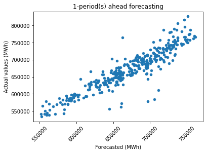
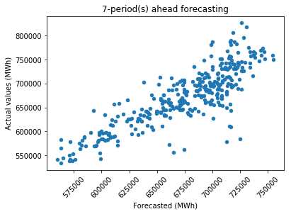
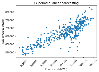
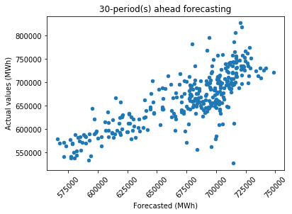
It is evident that as the forecasting period becomes longer, there is an increase in the scattering of data points, particularly for extreme values. Forecasting 30 days aheadOutput: 
Output: 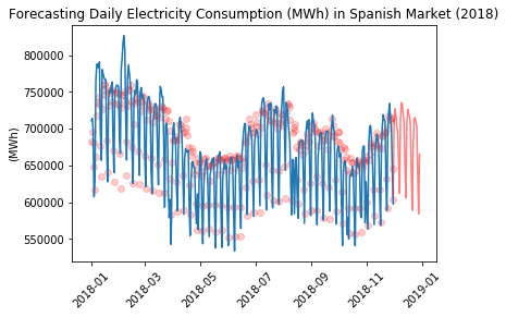
Future Aspects of Machine LearningMachine learning holds immense potential for the energy industry. By analyzing vast historical data, including electricity usage, weather patterns, and seasonal variations, machine learning algorithms can provide accurate predictions. Challenges such as complex relationships between variables are being addressed with advanced techniques. The future of this field looks promising, with improved accuracy, integration of IoT and smart grid data, and real-time predictive analytics. This will enable efficient energy distribution, demand-side response, and seamless integration of renewable energy sources. Moreover, machine learning will support predictive maintenance for energy infrastructure and foster energy conservation and sustainability. The collaboration between AI and human expertise will be essential, and transparent AI models will build trust and accountability. Overall, machine learning is set to transform the energy sector and pave the way for a more sustainable and efficient energy ecosystem. ConclusionElectricity consumption prediction using machine learning is a game-changer in the energy industry. By harnessing the power of data and advanced algorithms, we are unlocking new possibilities for efficient energy management and a greener tomorrow. As machine learning continues to evolve, we can look forward to a future where electricity consumption becomes more sustainable, economical, and environmentally friendly. Embracing this cutting-edge approach will pave the way for a brighter and more sustainable energy future.
Next TopicData Analytics vs. Machine Learning
|
 For Videos Join Our Youtube Channel: Join Now
Feedback
- Send your Feedback to [email protected]
Help Others, Please Share


