Apriori Algorithm in Machine Learning

The Apriori algorithm uses frequent itemsets to generate association rules, and it is designed to work on the databases that contain transactions. With the help of these association rule, it determines how strongly or how weakly two objects are connected. This algorithm uses a breadth-first search and Hash Tree to calculate the itemset associations efficiently. It is the iterative process for finding the frequent itemsets from the large dataset.

This algorithm was given by the R. Agrawal and Srikant in the year 1994. It is mainly used for market basket analysis and helps to find those products that can be bought together. It can also be used in the healthcare field to find drug reactions for patients.

What is Frequent Itemset?

Frequent itemsets are those items whose support is greater than the threshold value or user-specified minimum support. It means if A & B are the frequent itemsets together, then individually A and B should also be the frequent itemset.

Suppose there are the two transactions: A= {1,2,3,4,5}, and B= {2,3,7}, in these two transactions, 2 and 3 are the frequent itemsets.

Note: To better understand the apriori algorithm, and related term such as support and confidence, it is recommended to understand the association rule learning.

Steps for Apriori Algorithm

Below are the steps for the apriori algorithm:

Step-1: Determine the support of itemsets in the transactional database, and select the minimum support and confidence.

Step-2: Take all supports in the transaction with higher support value than the minimum or selected support value.

Step-3: Find all the rules of these subsets that have higher confidence value than the threshold or minimum confidence.

Step-4: Sort the rules as the decreasing order of lift.

Apriori Algorithm Working

We will understand the apriori algorithm using an example and mathematical calculation:

Example: Suppose we have the following dataset that has various transactions, and from this dataset, we need to find the frequent itemsets and generate the association rules using the Apriori algorithm: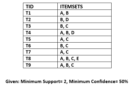

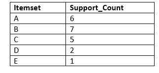
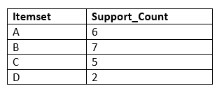
Solution:

Step-1: Calculating C1 and L1:

• In the first step, we will create a table that contains support count (The frequency of each itemset individually in the dataset) of each itemset in the given dataset. This table is called the Candidate set or C1.
  
• Now, we will take out all the itemsets that have the greater support count that the Minimum Support (2). It will give us the table for the frequent itemset L1.
  Since all the itemsets have greater or equal support count than the minimum support, except the E, so E itemset will be removed.
  

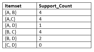
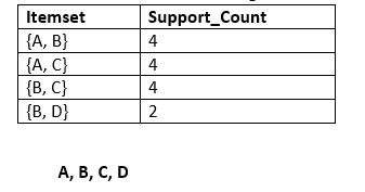
Step-2: Candidate Generation C2, and L2:

• In this step, we will generate C2 with the help of L1. In C2, we will create the pair of the itemsets of L1 in the form of subsets.
• After creating the subsets, we will again find the support count from the main transaction table of datasets, i.e., how many times these pairs have occurred together in the given dataset. So, we will get the below table for C2:
  
• Again, we need to compare the C2 Support count with the minimum support count, and after comparing, the itemset with less support count will be eliminated from the table C2. It will give us the below table for L2
  

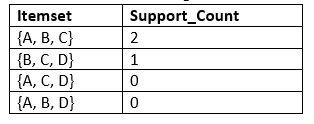
Step-3: Candidate generation C3, and L3:

• For C3, we will repeat the same two processes, but now we will form the C3 table with subsets of three itemsets together, and will calculate the support count from the dataset. It will give the below table:
  
• Now we will create the L3 table. As we can see from the above C3 table, there is only one combination of itemset that has support count equal to the minimum support count. So, the L3 will have only one combination, i.e., {A, B, C}.

Step-4: Finding the association rules for the subsets:

To generate the association rules, first, we will create a new table with the possible rules from the occurred combination {A, B.C}. For all the rules, we will calculate the Confidence using formula sup( A ^B)/A. After calculating the confidence value for all rules, we will exclude the rules that have less confidence than the minimum threshold(50%).

Consider the below table:

As the given threshold or minimum confidence is 50%, so the first three rules A ^B → C, B^C → A, and A^C → B can be considered as the strong association rules for the given problem.

Advantages of Apriori Algorithm

• This is easy to understand algorithm
• The join and prune steps of the algorithm can be easily implemented on large datasets.

Disadvantages of Apriori Algorithm

• The apriori algorithm works slow compared to other algorithms.
• The overall performance can be reduced as it scans the database for multiple times.
• The time complexity and space complexity of the apriori algorithm is O(2^D), which is very high. Here D represents the horizontal width present in the database.

Python Implementation of Apriori Algorithm

Now we will see the practical implementation of the Apriori Algorithm. To implement this, we have a problem of a retailer, who wants to find the association between his shop's product, so that he can provide an offer of "Buy this and Get that" to his customers.

The retailer has a dataset information that contains a list of transactions made by his customer. In the dataset, each row shows the products purchased by customers or transactions made by the customer. To solve this problem, we will perform the below steps:

• Data Pre-processing
• Training the Apriori model on the dataset
• Visualizing the results

1. Data Pre-processing Step:

The first step is data pre-processing step. Under this, first, we will perform the importing of the libraries. The code for this is given below:

• Importing the libraries:

Before importing the libraries, we will use the below line of code to install the apyori package to use further, as Spyder IDE does not contain it:

Below is the code to implement the libraries that will be used for different tasks of the model:

• Importing the dataset:
  Now, we will import the dataset for our apriori model. To import the dataset, there will be some changes here. All the rows of the dataset are showing different transactions made by the customers. The first row is the transaction done by the first customer, which means there is no particular name for each column and have their own individual value or product details(See the dataset given below after the code). So, we need to mention here in our code that there is no header specified. The code is given below:

In the above code, the first line is showing importing the dataset into pandas format. The second line of the code is used because the apriori() that we will use for training our model takes the dataset in the format of the list of the transactions. So, we have created an empty list of the transaction. This list will contain all the itemsets from 0 to 7500. Here we have taken 7501 because, in Python, the last index is not considered.

The dataset looks like the below image: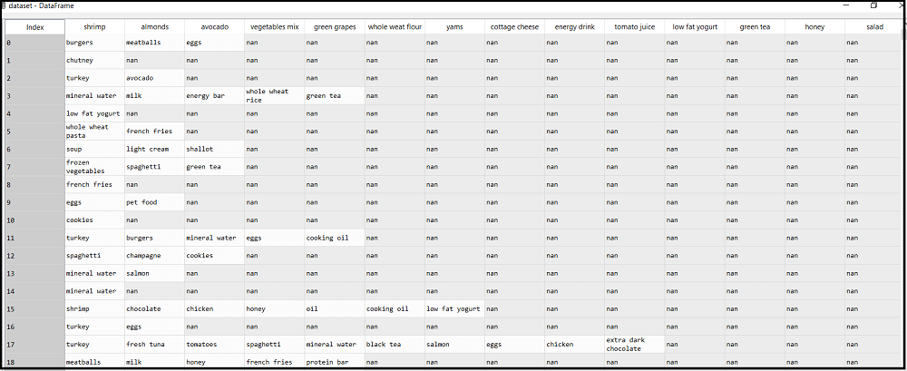

2. Training the Apriori Model on the dataset

To train the model, we will use the apriori function that will be imported from the apyroi package. This function will return the rules to train the model on the dataset. Consider the below code:

In the above code, the first line is to import the apriori function. In the second line, the apriori function returns the output as the rules. It takes the following parameters:

• transactions: A list of transactions.
• min_support= To set the minimum support float value. Here we have used 0.003 that is calculated by taking 3 transactions per customer each week to the total number of transactions.
• min_confidence: To set the minimum confidence value. Here we have taken 0.2. It can be changed as per the business problem.
• min_lift= To set the minimum lift value.
• min_length= It takes the minimum number of products for the association.
• max_length = It takes the maximum number of products for the association.

3. Visualizing the result

Now we will visualize the output for our apriori model. Here we will follow some more steps, which are given below:

• Displaying the result of the rules occurred from the apriori function

By executing the above lines of code, we will get the 9 rules. Consider the below output:

Output:

[RelationRecord(items=frozenset({'chicken', 'light cream'}), support=0.004533333333333334, ordered_statistics=[OrderedStatistic(items_base=frozenset({'light cream'}), items_add=frozenset({'chicken'}), confidence=0.2905982905982906, lift=4.843304843304844)]),
 RelationRecord(items=frozenset({'escalope', 'mushroom cream sauce'}), support=0.005733333333333333, ordered_statistics=[OrderedStatistic(items_base=frozenset({'mushroom cream sauce'}), items_add=frozenset({'escalope'}), confidence=0.30069930069930073, lift=3.7903273197390845)]),
 RelationRecord(items=frozenset({'escalope', 'pasta'}), support=0.005866666666666667, ordered_statistics=[OrderedStatistic(items_base=frozenset({'pasta'}), items_add=frozenset({'escalope'}), confidence=0.37288135593220345, lift=4.700185158809287)]),
 RelationRecord(items=frozenset({'fromage blanc', 'honey'}), support=0.0033333333333333335, ordered_statistics=[OrderedStatistic(items_base=frozenset({'fromage blanc'}), items_add=frozenset({'honey'}), confidence=0.2450980392156863, lift=5.178127589063795)]),
 RelationRecord(items=frozenset({'ground beef', 'herb & pepper'}), support=0.016, ordered_statistics=[OrderedStatistic(items_base=frozenset({'herb & pepper'}), items_add=frozenset({'ground beef'}), confidence=0.3234501347708895, lift=3.2915549671393096)]),
 RelationRecord(items=frozenset({'tomato sauce', 'ground beef'}), support=0.005333333333333333, ordered_statistics=[OrderedStatistic(items_base=frozenset({'tomato sauce'}), items_add=frozenset({'ground beef'}), confidence=0.37735849056603776, lift=3.840147461662528)]),
 RelationRecord(items=frozenset({'olive oil', 'light cream'}), support=0.0032, ordered_statistics=[OrderedStatistic(items_base=frozenset({'light cream'}), items_add=frozenset({'olive oil'}), confidence=0.20512820512820515, lift=3.120611639881417)]),
 RelationRecord(items=frozenset({'olive oil', 'whole wheat pasta'}), support=0.008, ordered_statistics=[OrderedStatistic(items_base=frozenset({'whole wheat pasta'}), items_add=frozenset({'olive oil'}), confidence=0.2714932126696833, lift=4.130221288078346)]),
 RelationRecord(items=frozenset({'pasta', 'shrimp'}), support=0.005066666666666666, ordered_statistics=[OrderedStatistic(items_base=frozenset({'pasta'}), items_add=frozenset({'shrimp'}), confidence=0.3220338983050848, lift=4.514493901473151)])]

As we can see, the above output is in the form that is not easily understandable. So, we will print all the rules in a suitable format.

• Visualizing the rule, support, confidence, lift in more clear way:

Output:

By executing the above lines of code, we will get the below output:

Rule: chicken -> light cream
Support: 0.004533333333333334
Confidence: 0.2905982905982906
Lift: 4.843304843304844
=====================================
Rule: escalope -> mushroom cream sauce
Support: 0.005733333333333333
Confidence: 0.30069930069930073
Lift: 3.7903273197390845
=====================================
Rule: escalope -> pasta
Support: 0.005866666666666667
Confidence: 0.37288135593220345
Lift: 4.700185158809287
=====================================
Rule: fromage blanc -> honey
Support: 0.0033333333333333335
Confidence: 0.2450980392156863
Lift: 5.178127589063795
=====================================
Rule: ground beef -> herb & pepper
Support: 0.016
Confidence: 0.3234501347708895
Lift: 3.2915549671393096
=====================================
Rule: tomato sauce -> ground beef
Support: 0.005333333333333333
Confidence: 0.37735849056603776
Lift: 3.840147461662528
=====================================
Rule: olive oil -> light cream
Support: 0.0032
Confidence: 0.20512820512820515
Lift: 3.120611639881417
=====================================
Rule: olive oil -> whole wheat pasta
Support: 0.008
Confidence: 0.2714932126696833
Lift: 4.130221288078346
=====================================
Rule: pasta -> shrimp
Support: 0.005066666666666666
Confidence: 0.3220338983050848
Lift: 4.514493901473151
=====================================

From the above output, we can analyze each rule. The first rules, which is Light cream → chicken, states that the light cream and chicken are bought frequently by most of the customers. The support for this rule is 0.0045, and the confidence is 29%. Hence, if a customer buys light cream, it is 29% chances that he also buys chicken, and it is .0045 times appeared in the transactions. We can check all these things in other rules also.