What are LSTM Networks

This tutorial discusses the issues with conventional RNNs resulting from increasing and decreasing gradients. It also proposes a solution that solves these problems through Long Short-Term Memory (LSTM). LST Memory is a sophisticated version of the recurrent neural networks (RNN) design that was created to represent chronological sequences and their long-range dependencies more precisely than traditional RNNs. Its main features are the internal design of an LSTM cell and the various modifications introduced into the LSTM structure, and a few applications of LSTMs that are in high demand. The article also provides an examination of LSTMs as well as GRUs. The tutorial ends with a list that outlines the drawbacks associated with the LSTM network and a description of the new models based on attention, which are swiftly replacing LSTMs in the real world.

Introduction:

LSTM networks extend the recurrent neural network (RNNs) mainly designed to deal with situations in which RNNs do not work. When we talk about RNN, it is an algorithm that processes the current input by taking into account the output of previous events (feedback) and then storing it in the memory of its users for a brief amount of time (short-term memory). Of the many applications, its most well-known ones are those in the areas of non-Markovian speech control and music composition. However, there are some drawbacks to RNNs. It is the first to fail to save information over long periods of time. Sometimes an ancestor of data stored a considerable time ago is needed to determine the output of the present. However, RNNs are utterly incapable of managing these "long-term dependencies." The second issue is that there is no better control of which component of the context is required to continue and what part of the past must be forgotten. Other issues associated with RNNs are the exploding or disappearing slopes (explained later) that occur in training an RNN through backtracking. Therefore, the Long-Short-Term Memory (LSTM) was introduced into the picture. It was designed so that the problem of the gradient disappearing is eliminated almost entirely as the training model is unaffected. Long-time lags within specific issues are solved using LSTMs, which also deal with the effects of noise, distributed representations, or endless numbers. With LSTMs, they do not meet the requirement to maintain the same number of states before the time required by the hideaway Markov model (HMM). LSTMs offer us an extensive range of parameters like learning rates and output and input biases. Therefore, there is no need for minor adjustments. The effort to update each weight is decreased to O(1) by using LSTMs like those used in Back Propagation Through Time (BPTT), which is a significant advantage.

Exploding and Vanishing Gradients:

In training a network, the primary objective is to reduce the losses (in terms of cost or error) seen in the output of the network when training data is passed through it. We determine the gradient, or loss in relation to a weight set, then adjust the weights in accordance with this, and repeat this process until we arrive at an optimal set of weights that will ensure the loss is as low as. This is the idea behind reverse-tracking. Sometimes, it is the case that the gradient becomes minimal. It is important to note that the amount of gradient in one layer is determined by some aspects of the following layers. If any component is tiny (less one), The result is that the gradient will appear smaller. This is also known as "the scaling effect. If this effect is multiplied by the rate of learning, which is a tiny value that ranges from 0.1-to 0.001, this produces a lower value. This means that the change in weights is minimal and produces nearly the same results as before. If the gradients are significant because of the vast components and the weights are changed to be higher than the ideal value. The issue is commonly referred to as the issue of explosive gradients. To stop this effect of scaling, the neural network unit was rebuilt such that the scale factor was set to one. The cell was then enhanced by a number of gating units and was named the LSTM.

Architecture:

The main difference between the structures that comprise RNNs as well as LSTMs can be seen in the fact that the hidden layer of LSTM is the gated unit or cell. It has four layers that work with each other to create the output of the cell, as well as the cell's state. Both of these are transferred to the next layer. Contrary to RNNs, which comprise the sole neural net layer made up of Tanh, LSTMs are comprised of three logistic sigmoid gates and a Tanh layer. Gates were added to restrict the information that goes through cells. They decide which portion of the data is required in the next cell and which parts must be eliminated. The output will typically fall in the range of 0-1, where "0" is a reference to "reject all' while "1" means "include all."

Hidden layers of LSTM: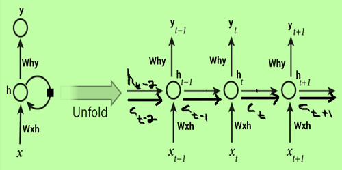

Each LSTM cell is equipped with three inputs and two outputs, h_t, and C_t. At a specific time, t, which h_t is the hidden state, and C_t is the cell state or memory. It x_t is the present information point or the input. The first sigmoid layer contains two inputs: h_t-1 and x_t, where h_t-1 is the state hidden in the cell before it. It is also known by its name and the forget gate since its output is a selection of the amount of data from the last cell that should be included. Its output will be a number [0,1] multiplied (pointwise) by the previous cell's state .

Applications:

LSTM models have to be trained using a training dataset before being used for real-world use. The most challenging applications are listed in the following sections:

1. Text generation or language modelling involves the calculation of words whenever a sequence of words is supplied as input. Language models can be used at the level of characters or n-gram level as well as at the sentence or the level of a paragraph.
2. Image processing is the process of the analysis of a photograph and converting the result into sentences. In order to do this, we will need to have a set of data consisting of many photos with the appropriate descriptive captions. A model that has been trained can determine the characteristics of images in the data. It is a photo dataset. The data is processed to include only those words that suggest the most. It is text data. By combining these two types of information, we will try to make the model work. The model's job is to produce a descriptive phrase for the image, one word at the moment, using input words predicted by the model and the image.
3. Speech and Handwriting Recognition
4. The process of music generation is identical to text generation, where LSTMs can predict the musical notes, not text, by studying a mix of notes fed into the input.
5. Language Translation involves translating a sequence of one language to a similar sequence in a different language. Like image processing, an image-based dataset that includes words and translations is cleaned first before the relevant portion to build the model. An encoder-decoder LSTM model can convert the input sequences into their formatted vector (encoding) and then convert the translated version.

Drawbacks:

Everything in the world indeed has its advantages and disadvantages. LSTMs are no exception, and they also come with a few disadvantages that are discussed below:

1. They became popular due to the fact that they solved the issue of gradients disappearing. However that they are unable to eliminate the problem. The issue lies in that data needs to be moved between cells for its analysis. Furthermore, the cell is becoming extremely complex with the addition of functions (such as the forget gate) that are now part of the picture.
2. They require lots of time and resources to be trained and prepared for real-world applications. Technically speaking, they require high memory bandwidth due to the linear layers present within each cell, which the system is usually unable to supply. Therefore, in terms of hardware, LSTMs become pretty inefficient.
3. With the growing technology of data, mining scientists are searching for a system that is able to store past data for more extended periods of time than LSTMs. The motivation behind the development of such a model is the habit of humans of dividing a particular chunk of information into smaller parts to facilitate recollection.
4. LSTMs are affected by various random weights and behave similarly to neural networks that feed forward. They favour small initialization over large weights.
5. LSTMs tend to overfit, and it can be challenging to implement dropout to stop this problem. Dropout is a method of regularization that ensures that inputs and recurrent connectivity with LSTM units are systematically exempted from weight updates and activation when developing a network.