Logistic Regression in Machine Learning

• Logistic regression is one of the most popular Machine Learning algorithms, which comes under the Supervised Learning technique. It is used for predicting the categorical dependent variable using a given set of independent variables.
• Logistic regression predicts the output of a categorical dependent variable. Therefore the outcome must be a categorical or discrete value. It can be either Yes or No, 0 or 1, true or False, etc. but instead of giving the exact value as 0 and 1, it gives the probabilistic values which lie between 0 and 1.
• Logistic Regression is much similar to the Linear Regression except that how they are used. Linear Regression is used for solving Regression problems, whereas Logistic regression is used for solving the classification problems.
• In Logistic regression, instead of fitting a regression line, we fit an "S" shaped logistic function, which predicts two maximum values (0 or 1).
• The curve from the logistic function indicates the likelihood of something such as whether the cells are cancerous or not, a mouse is obese or not based on its weight, etc.
• Logistic Regression is a significant machine learning algorithm because it has the ability to provide probabilities and classify new data using continuous and discrete datasets.
• Logistic Regression can be used to classify the observations using different types of data and can easily determine the most effective variables used for the classification. The below image is showing the logistic function:

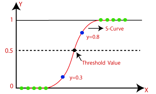
Note: Logistic regression uses the concept of predictive modeling as regression; therefore, it is called logistic regression, but is used to classify samples; Therefore, it falls under the classification algorithm.

Logistic Function (Sigmoid Function):

• The sigmoid function is a mathematical function used to map the predicted values to probabilities.
• It maps any real value into another value within a range of 0 and 1.
• The value of the logistic regression must be between 0 and 1, which cannot go beyond this limit, so it forms a curve like the "S" form. The S-form curve is called the Sigmoid function or the logistic function.
• In logistic regression, we use the concept of the threshold value, which defines the probability of either 0 or 1. Such as values above the threshold value tends to 1, and a value below the threshold values tends to 0.

Assumptions for Logistic Regression:

• The dependent variable must be categorical in nature.
• The independent variable should not have multi-collinearity.

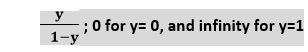
Logistic Regression Equation:

The Logistic regression equation can be obtained from the Linear Regression equation. The mathematical steps to get Logistic Regression equations are given below:

• We know the equation of the straight line can be written as:

• In Logistic Regression y can be between 0 and 1 only, so for this let's divide the above equation by (1-y):

• But we need range between -[infinity] to +[infinity], then take logarithm of the equation it will become:

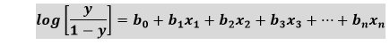
The above equation is the final equation for Logistic Regression.

Type of Logistic Regression:

On the basis of the categories, Logistic Regression can be classified into three types:

• Binomial: In binomial Logistic regression, there can be only two possible types of the dependent variables, such as 0 or 1, Pass or Fail, etc.
• Multinomial: In multinomial Logistic regression, there can be 3 or more possible unordered types of the dependent variable, such as "cat", "dogs", or "sheep"
• Ordinal: In ordinal Logistic regression, there can be 3 or more possible ordered types of dependent variables, such as "low", "Medium", or "High".

Python Implementation of Logistic Regression (Binomial)

To understand the implementation of Logistic Regression in Python, we will use the below example:

Example: There is a dataset given which contains the information of various users obtained from the social networking sites. There is a car making company that has recently launched a new SUV car. So the company wanted to check how many users from the dataset, wants to purchase the car.

For this problem, we will build a Machine Learning model using the Logistic regression algorithm. The dataset is shown in the below image. In this problem, we will predict the purchased variable (Dependent Variable) by using age and salary (Independent variables).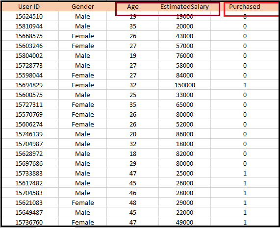

Steps in Logistic Regression: To implement the Logistic Regression using Python, we will use the same steps as we have done in previous topics of Regression. Below are the steps:

• Data Pre-processing step
• Fitting Logistic Regression to the Training set
• Predicting the test result
• Test accuracy of the result(Creation of Confusion matrix)
• Visualizing the test set result.

1. Data Pre-processing step: In this step, we will pre-process/prepare the data so that we can use it in our code efficiently. It will be the same as we have done in Data pre-processing topic. The code for this is given below:

By executing the above lines of code, we will get the dataset as the output. Consider the given image: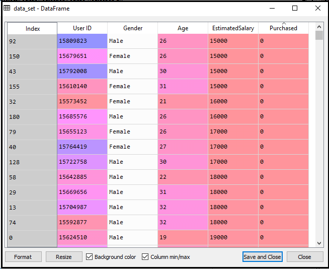

Now, we will extract the dependent and independent variables from the given dataset. Below is the code for it:

In the above code, we have taken [2, 3] for x because our independent variables are age and salary, which are at index 2, 3. And we have taken 4 for y variable because our dependent variable is at index 4. The output will be: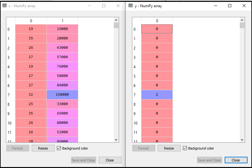

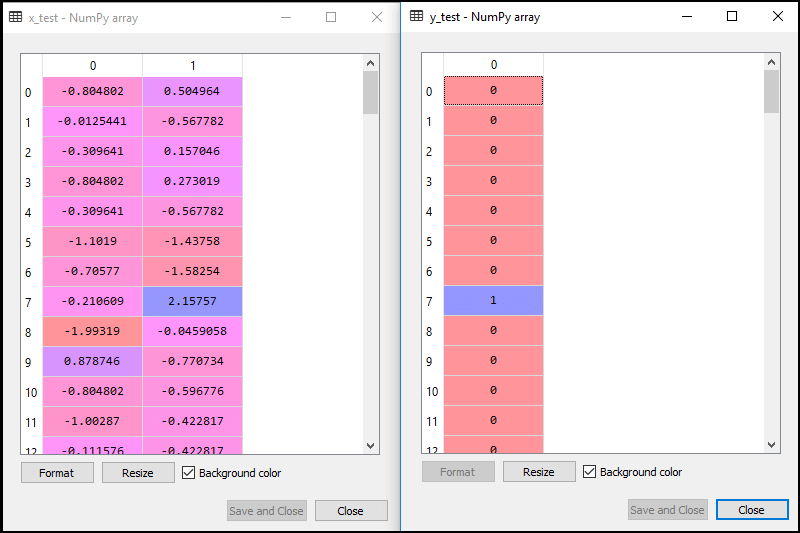
Now we will split the dataset into a training set and test set. Below is the code for it:

The output for this is given below:

For test set:

For training set:

In logistic regression, we will do feature scaling because we want accurate result of predictions. Here we will only scale the independent variable because dependent variable have only 0 and 1 values. Below is the code for it:

The scaled output is given below: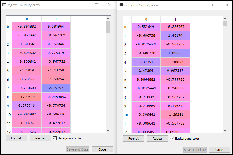

2. Fitting Logistic Regression to the Training set:

We have well prepared our dataset, and now we will train the dataset using the training set. For providing training or fitting the model to the training set, we will import the LogisticRegression class of the sklearn library.

After importing the class, we will create a classifier object and use it to fit the model to the logistic regression. Below is the code for it:

Output: By executing the above code, we will get the below output:

Out[5]:

Hence our model is well fitted to the training set.

3. Predicting the Test Result

Our model is well trained on the training set, so we will now predict the result by using test set data. Below is the code for it:

In the above code, we have created a y_pred vector to predict the test set result.

Output: By executing the above code, a new vector (y_pred) will be created under the variable explorer option. It can be seen as: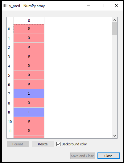

The above output image shows the corresponding predicted users who want to purchase or not purchase the car.

4. Test Accuracy of the result

Now we will create the confusion matrix here to check the accuracy of the classification. To create it, we need to import the confusion_matrix function of the sklearn library. After importing the function, we will call it using a new variable cm. The function takes two parameters, mainly y_true( the actual values) and y_pred (the targeted value return by the classifier). Below is the code for it:

Output:

By executing the above code, a new confusion matrix will be created. Consider the below image: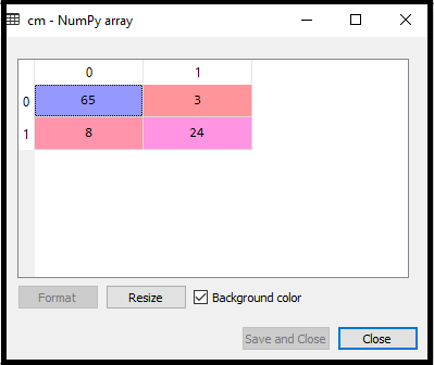

We can find the accuracy of the predicted result by interpreting the confusion matrix. By above output, we can interpret that 65+24= 89 (Correct Output) and 8+3= 11(Incorrect Output).

5. Visualizing the training set result

Finally, we will visualize the training set result. To visualize the result, we will use ListedColormap class of matplotlib library. Below is the code for it:

In the above code, we have imported the ListedColormap class of Matplotlib library to create the colormap for visualizing the result. We have created two new variables x_set and y_set to replace x_train and y_train. After that, we have used the nm.meshgrid command to create a rectangular grid, which has a range of -1(minimum) to 1 (maximum). The pixel points we have taken are of 0.01 resolution.

To create a filled contour, we have used mtp.contourf command, it will create regions of provided colors (purple and green). In this function, we have passed the classifier.predict to show the predicted data points predicted by the classifier.

Output: By executing the above code, we will get the below output: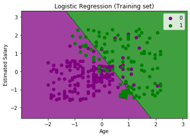

The graph can be explained in the below points:

• In the above graph, we can see that there are some Green points within the green region and Purple points within the purple region.
• All these data points are the observation points from the training set, which shows the result for purchased variables.
• This graph is made by using two independent variables i.e., Age on the x-axis and Estimated salary on the y-axis.
• The purple point observations are for which purchased (dependent variable) is probably 0, i.e., users who did not purchase the SUV car.
• The green point observations are for which purchased (dependent variable) is probably 1 means user who purchased the SUV car.
• We can also estimate from the graph that the users who are younger with low salary, did not purchase the car, whereas older users with high estimated salary purchased the car.
• But there are some purple points in the green region (Buying the car) and some green points in the purple region(Not buying the car). So we can say that younger users with a high estimated salary purchased the car, whereas an older user with a low estimated salary did not purchase the car.

The goal of the classifier:

We have successfully visualized the training set result for the logistic regression, and our goal for this classification is to divide the users who purchased the SUV car and who did not purchase the car. So from the output graph, we can clearly see the two regions (Purple and Green) with the observation points. The Purple region is for those users who didn't buy the car, and Green Region is for those users who purchased the car.

Linear Classifier:

As we can see from the graph, the classifier is a Straight line or linear in nature as we have used the Linear model for Logistic Regression. In further topics, we will learn for non-linear Classifiers.

Visualizing the test set result:

Our model is well trained using the training dataset. Now, we will visualize the result for new observations (Test set). The code for the test set will remain same as above except that here we will use x_test and y_test instead of x_train and y_train. Below is the code for it:

Output: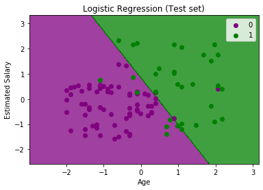

The above graph shows the test set result. As we can see, the graph is divided into two regions (Purple and Green). And Green observations are in the green region, and Purple observations are in the purple region. So we can say it is a good prediction and model. Some of the green and purple data points are in different regions, which can be ignored as we have already calculated this error using the confusion matrix (11 Incorrect output).

Hence our model is pretty good and ready to make new predictions for this classification problem.