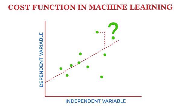
Cost Function in Machine Learning

A Machine Learning model should have a very high level of accuracy in order to perform well with real-world applications. But how to calculate the accuracy of the model, i.e., how good or poor our model will perform in the real world? In such a case, the Cost function comes into existence. It is an important machine learning parameter to correctly estimate the model.

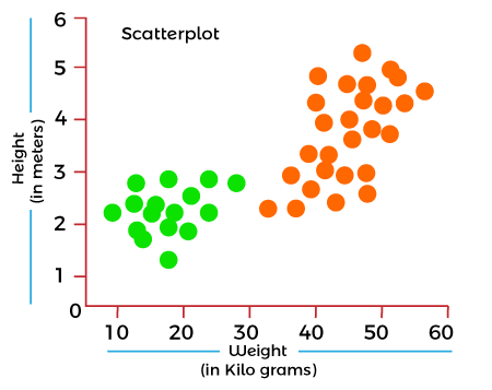
Cost function also plays a crucial role in understanding that how well your model estimates the relationship between the input and output parameters.

In this topic, we will explain the cost function in Machine Learning, Gradient descent, and types of cost functions.

What is Cost Function?

A cost function is an important parameter that determines how well a machine learning model performs for a given dataset. It calculates the difference between the expected value and predicted value and represents it as a single real number.

In machine learning, once we train our model, then we want to see how well our model is performing. Although there are various accuracy functions that tell you how your model is performing, but will not give insights to improve them. So, we need a function that can find when the model is most accurate by finding the spot between the undertrained and overtrained model.

In simple, "Cost function is a measure of how wrong the model is in estimating the relationship between X(input) and Y(output) Parameter." A cost function is sometimes also referred to as Loss function, and it can be estimated by iteratively running the model to compare estimated predictions against the known values of Y.

The main aim of each ML model is to determine parameters or weights that can minimize the cost function.

Why use Cost Function?

While there are different accuracy parameters, then why do we need a Cost function for the Machine learning model. So, we can understand it with an example of the classification of data. Suppose we have a dataset that contains the height and weights of cats & dogs, and we need to classify them accordingly. If we plot the records using these two features, we will get a scatter plot as below:

In the above image, the green dots are cats, and the yellow dots are dogs. Below are the three possible solutions for this classification problem.

In the above solutions, all three classifiers have high accuracy, but the third solution is the best because it correctly classifies each datapoint. The reason behind the best classification is that it is in mid between both the classes, not close or not far to any of them.

To get such results, we need a Cost function. It means for getting the optimal solution; we need a Cost function. It calculated the difference between the actual values and predicted values and measured how wrong was our model in the prediction. By minimizing the value of the cost function, we can get the optimal solution.

Gradient Descent: Minimizing the cost function

As we discussed in the above section, the cost function tells how wrong your model is? And each machine learning model tries to minimize the cost function in order to give the best results. Here comes the role of Gradient descent.

"Gradient Descent is an optimization algorithm which is used for optimizing the cost function or error in the model." It enables the models to take the gradient or direction to reduce the errors by reaching to least possible error. Here direction refers to how model parameters should be corrected to further reduce the cost function. The error in your model can be different at different points, and you have to find the quickest way to minimize it, to prevent resource wastage.

Gradient descent is an iterative process where the model gradually converges towards a minimum value, and if the model iterates further than this point, it produces little or zero changes in the loss. This point is known as convergence, and at this point, the error is least, and the cost function is optimized.

Below is the equation for gradient descent in linear regression:

In the gradient descent equation, alpha is known as the learning rate. This parameter decides how fast you should move down to the slope. For large alpha, take big steps, and for small alpha value, you need to take small steps.

Types of Cost Function

Cost functions can be of various types depending on the problem. However, mainly it is of three types, which are as follows:

1. Regression Cost Function
2. Binary Classification cost Functions
3. Multi-class Classification Cost Function.

1. Regression Cost Function

Regression models are used to make a prediction for the continuous variables such as the price of houses, weather prediction, loan predictions, etc. When a cost function is used with Regression, it is known as the "Regression Cost Function." In this, the cost function is calculated as the error based on the distance, such as:

There are three commonly used Regression cost functions, which are as follows:

a. Means Error

In this type of cost function, the error is calculated for each training data, and then the mean of all error values is taken.

It is one of the simplest ways possible.

The errors that occurred from the training data can be either negative or positive. While finding mean, they can cancel out each other and result in the zero-mean error for the model, so it is not recommended cost function for a model.

However, it provides a base for other cost functions of regression models.

b. Mean Squared Error (MSE)

Means Square error is one of the most commonly used Cost function methods. It improves the drawbacks of the Mean error cost function, as it calculates the square of the difference between the actual value and predicted value. Because of the square of the difference, it avoids any possibility of negative error.

The formula for calculating MSE is given below:

Mean squared error is also known as L2 Loss.

In MSE, each error is squared, and it helps in reducing a small deviation in prediction as compared to MAE. But if the dataset has outliers that generate more prediction errors, then squaring of this error will further increase the error multiple times. Hence, we can say MSE is less robust to outliers.

c. Mean Absolute Error (MAE)

Mean Absolute error also overcome the issue of the Mean error cost function by taking the absolute difference between the actual value and predicted value.

The formula for calculating Mean Absolute Error is given below:

This means the Absolute error cost function is also known as L1 Loss. It is not affected by noise or outliers, hence giving better results if the dataset has noise or outlier.

2. Binary Classification Cost Functions

Classification models are used to make predictions of categorical variables, such as predictions for 0 or 1, Cat or dog, etc. The cost function used in the classification problem is known as the Classification cost function. However, the classification cost function is different from the Regression cost function.

One of the commonly used loss functions for classification is cross-entropy loss.

The binary Cost function is a special case of Categorical cross-entropy, where there is only one output class. For example, classification between red and blue.

To better understand it, let's suppose there is only a single output variable Y

The error in binary classification is calculated as the mean of cross-entropy for all N training data. Which means:

3. Multi-class Classification Cost Function

A multi-class classification cost function is used in the classification problems for which instances are allocated to one of more than two classes. Here also, similar to binary class classification cost function, cross-entropy or categorical cross-entropy is commonly used cost function.

It is designed in a way that it can be used with multi-class classification with the target values ranging from 0 to 1, 3, ….,n classes.

In a multi-class classification problem, cross-entropy will generate a score that summarizes the mean difference between actual and anticipated probability distribution.

For a perfect cross-entropy, the value should be zero when the score is minimized.