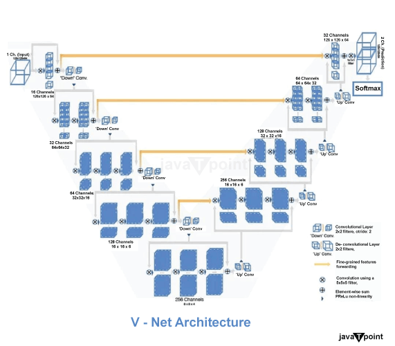
V-Net in Image SegmentationIntroduction:In this tutorial, we are learning about V-Net in Image Segmentation. V stands for virtual network. V-Net is reviewed. The most common clinical data in clinical practice include 3D volumes, like MRI volumes showing the prostate. However, most of the methods can only produce 2D images. Medical volume annotation is very tough. Professionals must do the annotation, which is very expensive. However, automatic Segmentation helps reduce costs. What is meant by Image Segmentation?Image segmentation is mainly used to detect any object. Here, we can mark the presence of objects by the pixel-level masks created for each object in an image. This process is more than just a difference between box generation. Because it helps us identify the shape of all objects in the image. Instead of drawing a bounding box, Segmentation helps identify the pixels that make up that object. This level of detail helps us with everything from image processing to satellite imagery. Recently, many image segmentation methods have been proposed. But the most popular of these is Mask R-CNN. It was introduced in 2017 by K He et al. Image Segmentation is mainly divided into two parts, which are given below - 1. Instance Segmentation: Instance Segmentation is a part of the Image Segmentation. Instance Segmentation means multiple instances of the same class are segmented separately. It means objects belonging to the same class are considered different. Therefore, all objects have different colors, even in the same class. 2. Semantic Segmentation: Semantic Segmentation is a part of the Image Segmentation. In semantic Segmentation, all types of objects belong to the same classification. So, all objects of the same class are colored with the same color. What is the difference between U-Net and V-Net?Here, we learn about the difference between V-Net and U-Net. The construction method of U-Net and V-Net is similar. It offers two different connection methods: the contracting method, which gradually removes the site's features and expands the extracted features to a specific location in the original image. The main idea of the building is the clock, then the two narrowing and widening roads meet halfway to form a clock. This model type provides accurate Segmentation based on output and is still one of the most widely used methods in computer vision today. Describe the architecture of V-Net.Here, we briefly learn about the architecture of the V-Net. V-Net architecture is shown in the below image. The left side of the network has a compressed path, while the right side decompresses the signal until it reaches its normal size. 
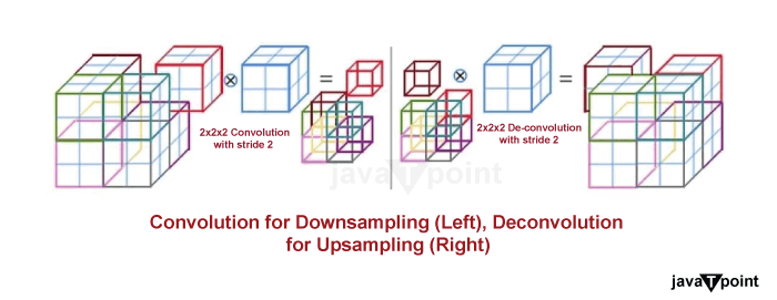
1. Left Side:The left side of the V-Net consists of various segments that have done various tasks. Each level has one to three convolution layers. A residual function is examined in each stage. The input for each level is used in a non-linearly obtained convolution layer, and this level can now learn its function in addition to the output of the last convolution layer. Compared to non-residual learning, such as U-Net, this model provides integration. Using the volumetric kernels, the convolution can be performed in each stage. The size of voxels is 5*5*5. According to the compression method, the resolution is reduced by convolution with a 2 × 2 × 2 voxel-wide kernel. Therefore, the resulting feature map is halved in size, and its purpose is like the pooling layer. The number of channels is doubled at each stage of the V-Net compression method. The pooling operation is replaced with a convolutional function. It helps reduce the memory footprint during training because backpropagation does not require switches that map the output of the pooling layer back to their host's input. The respective field can be increased by using down sampling. Basically, down Sampling is a process by which we small the digital signal by lowering the number of bits in the sample. Here, PreLU is used for the non-linear activation function. 2. Right Side:The right side of the V-Net consists of various segments that have done various tasks. The network extracts features and expands support for low-resolution feature maps to gather and aggregate the information needed to display the two-channel volume segmentation. The deconvolution operation is performed in each stage to increase the input size. This input is followed by convolution layers one to three. It consists of half of the 5×5×5 kernels used in the previous layer. 
Similar to the left side of the network, a residual function is learned. The last layer of convolution computes the two features' maps. It has a kernel size of 1×1×1 and produces output the same size as the input. The two output maps created are probabilistic segmentations of the foreground and background using soft-max voxels. Basically, up convolution is performed on the right side. 3. Connection in Horizontal:In the V-net architecture, we saw some horizontal connections there. In the compression path, the location information or data can be lost. This is similar to the U-Net. So, which features are extracted from the left side of the CNN, by using the horizontal connection, it can forward to the left side of the V-Net. The horizontal connection in the right part of the V-Net can provide the location information. The final contour prediction can be improved by it. The convergence time of the model can also be improved by using this connection horizontally. 4. Dice Loss:The dice loss formula D can be represented as a below - 
The dice coefficient D is placed between two binary volumes in the formula mentioned. The range of it belongs to 0 - 1. Here, N represents voxels, pi represents predicted, gi represents voxels and ground-truth voxels. As mentioned before, we get the output after SoftMax at the end of the networks. Here, each voxel of the networks belongs to the foreground and background. The dice coefficient D is differentiated, which is given in below - 
When the dice are rolled, there is no need to weigh samples from different classes to generate an equal number of leading and trailing voxels. 5. Results:Results are divided into two parts, which are training and testing. Now, we learn about these two parts in the below section - a. Training: All the volumes processed by the network have a size of 128 × 128 × 64 voxels. The resolution of it is 1 × 1 × 1.5 mm. The dataset is small because one or more experts need to track accurate location information and the costs associated with obtaining it. Subjects were trained using only 50 MRI volumes with realistic instructions from the PROMISE 2012 campaign dataset. Data augmentation is required here. A randomly deformed version of the training image is generated for each iteration using a dense deformation field obtained from the 2x2x2 control points and B-spline interpolation. For the requirement of high memory, the mini-batch only contains 2 volumes. The density of the data is varied using histogram matching to replace the density of the learning volume used at each iteration with another randomly selected dataset. b. Testing: The number of unseen volumes is 30, which is proceed here. After SoftMax, the voxels belong to the foreground with the highest probability to the background. It is considered as the anatomy part. In the testing section, we mainly measured the Hausdorff distance and the dice coefficient D. By the Hausdorff distance, we can measure the distance between two or more than two images.

The above table shows that V-Net with dice loss is better than V-Net with logistic loss. The V-Net outperforms existing technologies, not just Imorphics. Conclusion:So, by this tutorial, we are learning about V-Net in Image Segmentation. Image segmentation is mainly used to detect any object. V-Net basically a convolution of neural network. It is used of 3D image segmentation. Here, we learn image segmentation, V-Net, and V-Net architecture. V-Net Architecture consists two sides, which are left side and right side. Here we also learn about these sides. |
 For Videos Join Our Youtube Channel: Join Now
Feedback
- Send your Feedback to [email protected]
Help Others, Please Share


