Sentiment Analysis Using Machine Learning

Sentiment analysis, often referred to as opinion mining, is an intriguing field that leverages the capabilities of machine learning to comprehend and evaluate human emotions, attitudes, and viewpoints expressed in text data. In the fast-paced and dynamic digital world we live in, a vast amount of text is produced daily across diverse online platforms like social media, customer reviews, and feedback. For enterprises, researchers, and organizations, sentiment analysis has emerged as a crucial tool for gaining valuable insights into public sentiments and opinions. Understanding how people perceive and feel about products, services, or events has become essential in making informed decisions and staying ahead in this highly competitive landscape.

Using advanced language processing methods and machine learning algorithms, sentiment analysis can easily classify text into positive, negative, or neutral sentiments without any difficulty. This is accomplished by thoroughly examining patterns, contextual hints, and linguistic characteristics, empowering these models to accurately detect and evaluate the emotions expressed within the text.

Sentiment analysis can be categorized into several types, each with its own specific approach. For instance, document-level sentiment analysis aims to understand sentiments expressed throughout entire documents. On the other hand, sentence-level sentiment analysis hones in on individual sentences to grasp the emotions conveyed within them. Additionally, sub-sentence or phrase-level sentiment analysis delves into sentiments at a more granular level, providing a deeper understanding of the emotions behind smaller textual units.

Now we will try to do sentiment analysis on the movie review dataset.

Here, the sentiment labels are:

• 0 - negative
• 1 - somewhat negative
• 2 - neutral
• 3 - somewhat positive
• 4 - Positive

Sentiment Analysis in Machine Learning using Python

• Importing Libraries

• EDA (Exploratory Data Analysis)

Let's verify the count of examples and attributes present in the dataset.

Output:

Output: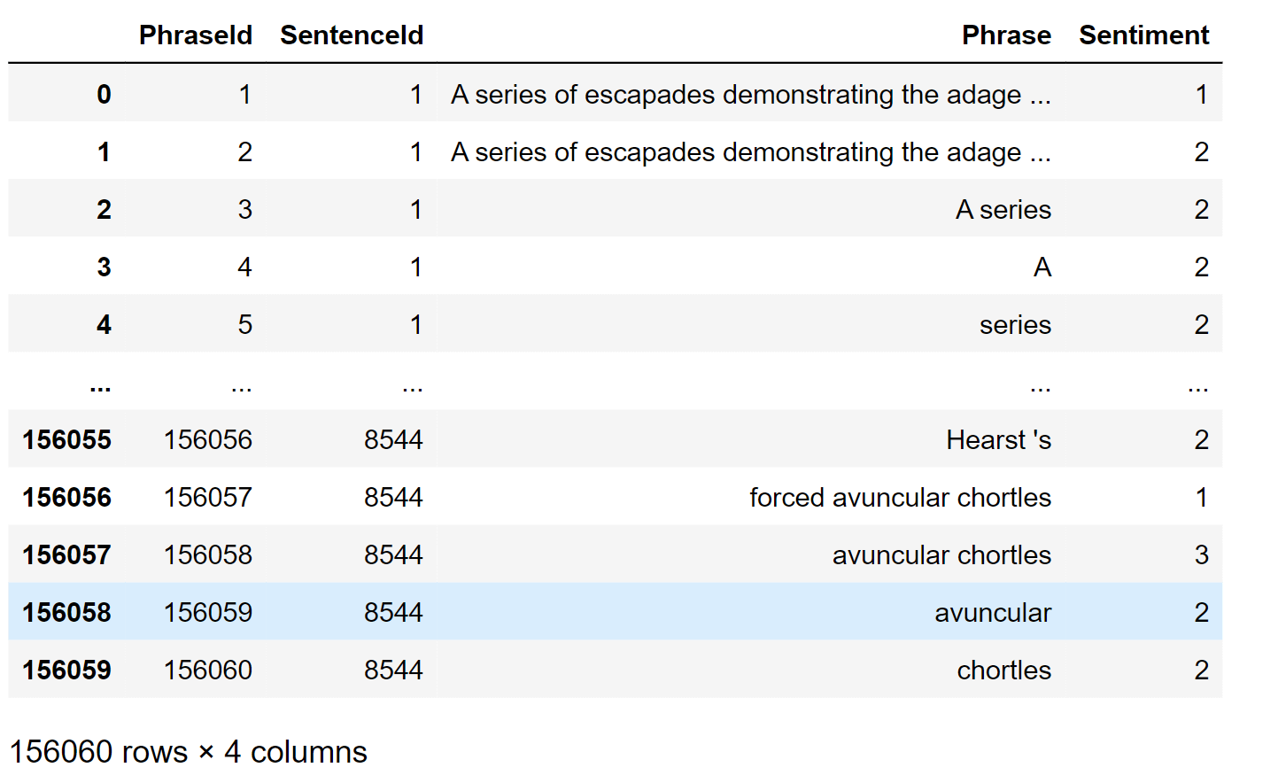

From the above, we observe that only the "Phrase" and "Sentiment" columns are required from the file for training the models later. Hence, we will utilize these as the feature (X) and label (Y) when fitting the transformer.

If there is any null or empty value in any column, we need to remove it. To identify such values, we will use the "info()" function.

Output: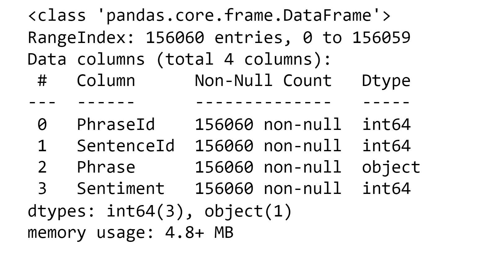

Output: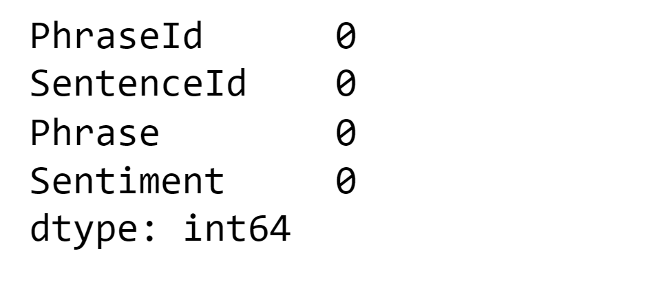

The dataset appears to be in good condition. It is important to examine how the five classes are distributed in the label to determine if it is balanced or not.

Output: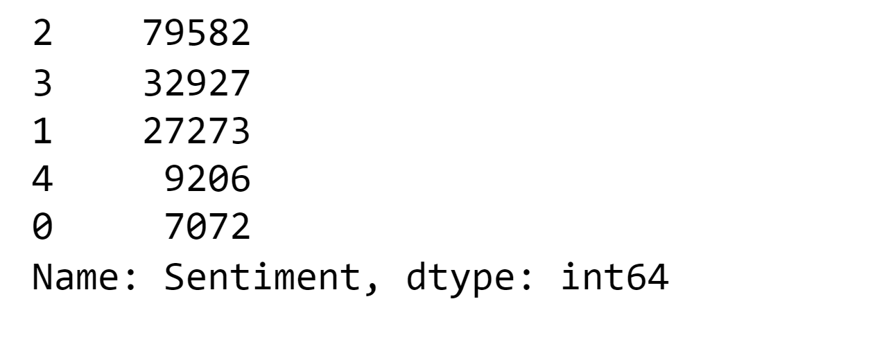

Output: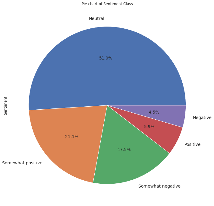

The distribution of the label is noticeably imbalanced, with only 'Neutral' representing more than 50% of instances and a slight skew towards positive reviews. This indicates that the class to be predicted will be biased towards the more frequent classes. Therefore, we will need a text balancing technique, such as 'SMOTE' for numerical features, to address this imbalance.

Let's proceed to determine the word count in the reviews to gain better insights. We will plot histograms for each class to understand the distribution more effectively.

Output: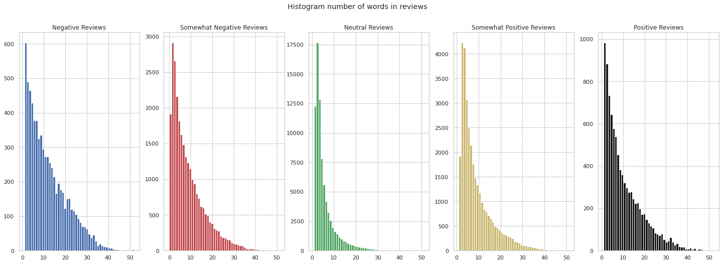

In the five histograms, we observe that the distribution follows a decreasing pattern that resembles a negative exponential function as we move along the x-axis. Notably, the class 'Negative Reviews' appears to have the longest sentences in the Phrase column, reaching approximately 52 words. To confirm the longest sentence, we will use the max() function.

Output:

Indeed, the longest sentence was 52 words. If we were to tokenize the text by words, the max_length should be set to 52. However, transformers utilize sub-word tokenization, which means the actual number of tokens could be higher, possibly reaching 60 or more, depending on the specific words used in the sentences. This aspect needs to be considered during the modeling process as it could significantly impact the training time. Finding a suitable trade-off between training time and performance is crucial to ensure efficient and effective model training.

Output:

We observe that 352 reviews have more than 40 words, and only 18 reviews exceed 50 words. These numbers represent a small fraction of the total instances (156,060), so setting limits based on them will not significantly impact the classification process. Below, we can find an example of a sentence containing 52 words. It's worth noting that the sentence includes misspelled words, acronyms, and some words that can be further broken down into sub-words.

Output:

• Modeling

Here, we will develop, train, and compare the following algorithms:

• BERT
• RoBERTa
• DistilBERT
• XLNet

Each of these models has its strengths and limitations. Among them, BERT is widely preferred and used due to its balanced performance. On the other hand, RoBERTa and others are known for achieving better error metrics, while DistilBERT stands out for its faster training speed. We will carefully consider all these characteristics to select the most suitable model for our dataset.

The necessary components required from `tensorflow.keras` are as follows:

Next, we will extract only the two relevant columns (Phrase and Sentiment) from the dataset for training purposes.

We will now divide the dataset into training and validation sets. Since the file contains over 150 thousand instances, we can choose a smaller portion for validation while still having a substantial number of instances. To achieve this, we will set the test_size to 10%.

BERT

To start, we need to import the necessary components for building the Bert model, including the Model, Config, and Tokenizer. These components are essential for constructing the model accurately.

We will utilize the 'bert_base_uncased' model, and the chosen max_length is set to 45 since there are only a few larger sequences in the dataset.

Output:

With our model loaded, we can now proceed to build and fine-tune it based on our dataset and task using the functional API of Keras. As depicted below, the input layer considers the max_length of sequences and then feeds it to the BERT model. A dropout layer is added with a rate of 0.1 to reduce overfitting, followed by a dense layer with the number of neurons equal to the number of classes in our label, which is 5.

Output: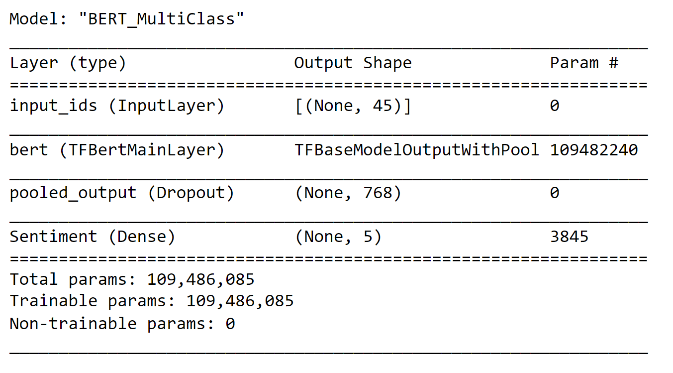

In the next step, we tokenize the training and validation sentences, set the label as categorical, and proceed with model training.

Output:

The model was trained for 2 epochs, and the training process took a total of 27 minutes and 20 seconds.

Evaluation on Validation Set

We will calculate the error metrics on the validation set to get an understanding of the model's performance.

Output:

Output:

Output: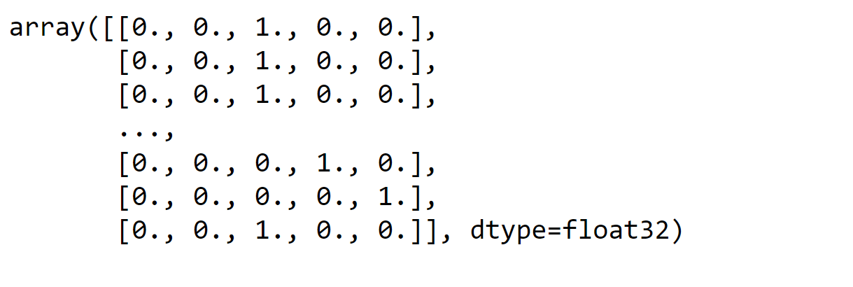

To generate the classification report and confusion matrix, we will convert the matrices into a single column representing the argmax for each row.

Output: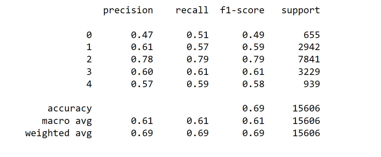

Due to the class imbalance in our dataset, our predictions are heavily biased towards the most frequent class, which in this case is class 2 ('Neutral'). As a result, the model's performance is subpar when it comes to predicting classes 0 or 4, rendering it nearly useless for this task. The significant number of misclassifications for these two classes is evident in the results below.

Output:

For the next three models, we will follow the same approach as the previous one, with some additional lines of code specific to each model.

Roberta

Output:

Output: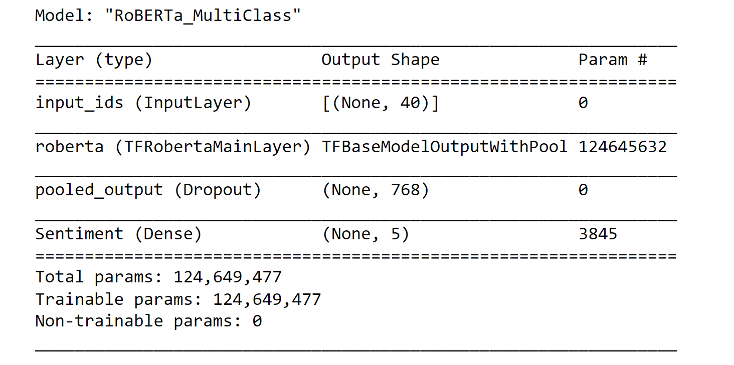

Output:

The model required 26 minutes to complete training for 2 epochs.

Evaluation on Validation Set

Output:

Output:

Output:

Output: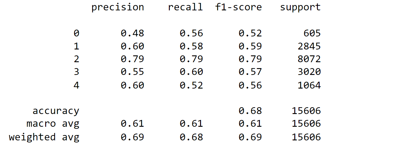

The overall accuracy of the model is 68%, with a weighted average F1 score of 69%. The macro-average F1-score, which considers all classes equally, is 61%. These metrics show that the model performs relatively well in predicting class 2 (Neutral), which is the most frequent class in the dataset. However, its performance is lower for classes 0 (Very Negative) and 4 (Very Positive), where precision and recall scores are not as high as desired. Further improvements may be required to enhance the model's accuracy and balance its predictions across all classes.

Output:

DitstilBert

Output:

In the default model of DistilBERT, there is no pooling layer that directly converts the output shape from (None, 45, 768) to (None, 768). To achieve the desired output shape, we will manually select the first and third dimensions of 'layer 0'. The subsequent layers will remain the same as before.

Output: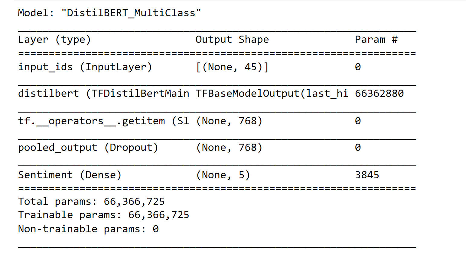

Output:

The model required 14 minutes to complete 2 epochs of training.

Evaluation on Validation Set

Output:

Output:

Output:

Output: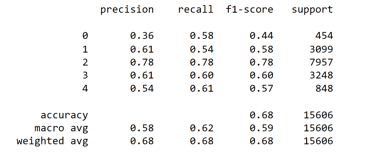

In this evaluation, the model achieves an accuracy of 68%, indicating that it makes correct predictions for 68% of the instances in the dataset. The precision, recall, and F1-score for each class are measures of the model's performance on classifying instances belonging to that class.

For class 0, the precision is 36%, indicating that when the model predicts instances as class 0, only 36% of them are correct. The recall is 58%, which means the model identifies 58% of the actual instances of class 0. The F1-score, which considers both precision and recall, is 44%.

Output:

XLNet

Output:

Similar to the DistilBERT model, the current model also requires converting the output shape of the default model's first layer to the desired shape of (None, 768). To achieve this, we utilize the tf.squeeze function.

Output: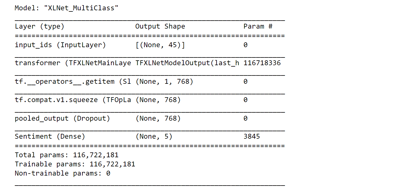

Output:

The model's training process lasted for 31 minutes and 16 seconds to complete 2 epochs.

Evaluation on Validation Set

Output:

Output:

Output: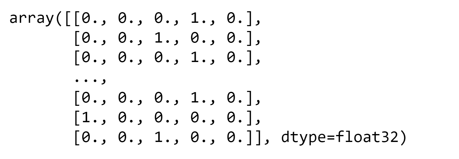

Output: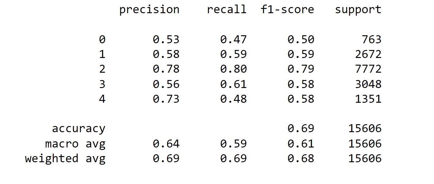

Overall, the model achieved an accuracy of 69% on the test set. Class 2, which corresponds to 'Neutral' sentiments, had the highest precision, recall, and F1-score, indicating good performance for this class. On the other hand, class 0 ('Very Negative') and class 4 ('Very Positive') had lower precision and recall values, suggesting that the model struggled to accurately predict these classes. The weighted average of all classes shows a balanced performance, but there is room for improvement, especially for the less frequent classes. The macro average, which takes into account the unbalanced nature of the dataset, shows an F1-score of 0.61, which indicates reasonable performance considering the class distribution.

Output: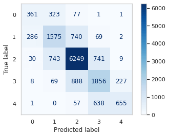

The performance of the four models was comparable, demonstrating that BERT strikes a balance between accuracy and training time. DistilBERT was notably the fastest model, but its accuracy was lower than the others, achieving around 95% accuracy compared to BERT. On the other hand, RoBERTa and XLNet exhibited the highest accuracy, albeit at the cost of longer training times. HuggingFace's explanation for DistilBERT's lower accuracy is that it achieves about 95% of BERT's accuracy.

Conclusion

Sentiment analysis using machine learning has emerged as a powerful tool for understanding human emotions and opinions expressed in text data. It finds applications in diverse fields, from marketing and customer service to political analysis and market research. As machine learning keeps progressing, the field of sentiment analysis is set to witness even greater precision and depth, providing valuable insights for informed decision-making and enriched user interactions. With the expansion of data availability and the ongoing enhancement of machine learning algorithms, sentiment analysis will continue to play a crucial role in deciphering the emotions of the digital realm. As technology evolves, the potential for sentiment analysis to deliver meaningful understandings will only grow, enriching our understanding of human sentiments in the digital space.