Sales Prediction Using Machine Learning

Machine learning is a powerful tool that can be used to predict sales and improve business outcomes. In this article, we will discuss how machine learning can be used to predict sales and the different methods that can be used to do so.

Machine Learning Methods for Sales Predcition

• One of the most common methods used to predict sales is regression analysis. This method involves using historical sales data to train a model that can predict future sales. The model can take into account factors such as past sales, marketing campaigns, and economic indicators to make its predictions.
• Another popular method for predicting sales is time series analysis. This method involves using historical sales data to identify patterns and trends in sales over time. The model can then use these patterns to make predictions about future sales. This method is particularly useful for predicting sales in seasonal industries, such as retail and tourism.
• Another approach is using decision tree-based algorithms like Random Forest, Gradient Boosting etc. These algorithms are particularly useful when there are many factors that can influence sales, such as product features, customer demographics, and market conditions. The algorithm can help identify the most important factors and use them to make predictions.
• In addition to these methods, machine learning can also be used to predict sales through the use of neural networks. Neural networks are a type of machine learning algorithm that can learn to recognize patterns in data. They can be trained on large amounts of sales data and can make predictions about future sales.
• Machine learning can also be used to predict sales by using clustering algorithms, which can help identify groups of similar customers. This information can then be used to create targeted marketing campaigns and improve sales strategies.

Sales Prediciton Using Python

So, now we will try to predict sales using various machine learning techniques.

Code:

1. Importing Libraries

2. Loading and Exploration of the Data

The data must first be loaded before being transformed into a structure that will be used by each of our models. Each row of data reflects a single day's worth of sales at one of 10 stores in its most basic form. Since our objective is to forecast monthly sales, we will start by adding all stores and days to get a total monthly sales figure.

Output: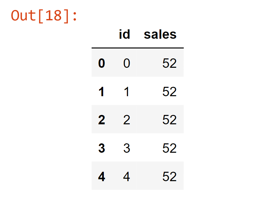

Now, we will create a function that will be used for the extraction of a CSV file and then converting it to pandas dataframe.

Output: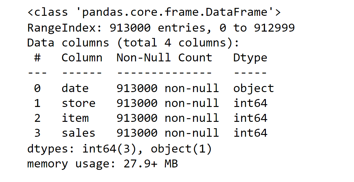

The above function returns a dataframe where each row represents total sales for a given month. Columns include 'date' by month and 'sales'.

Output: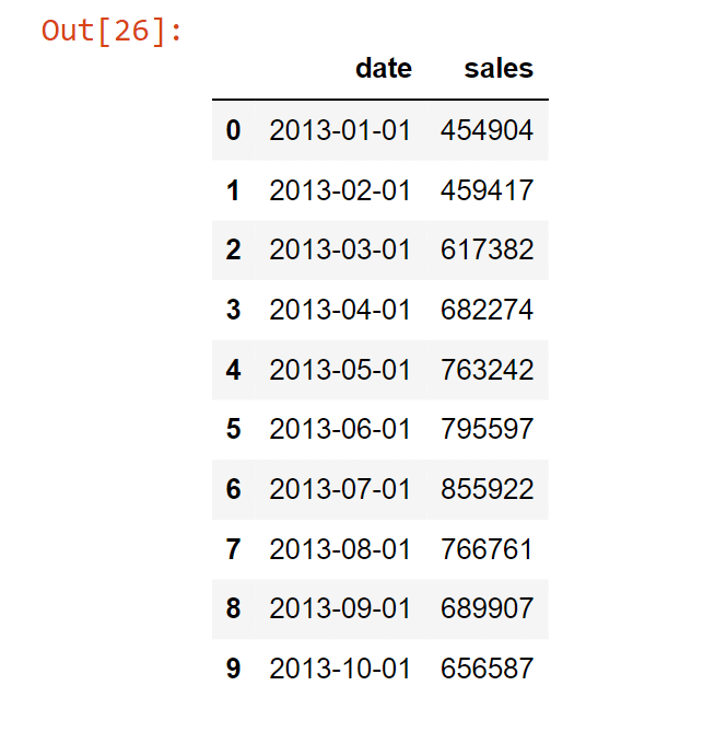

In the above data frame, each row now represents the total sales for a given month across stores.

Output: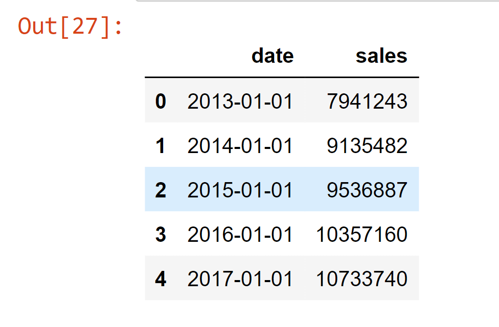

In the above data frame, each row now represents the total sales for a given year across stores.

Output:

<matplotlib.legend.Legend at 0x27280058fa0>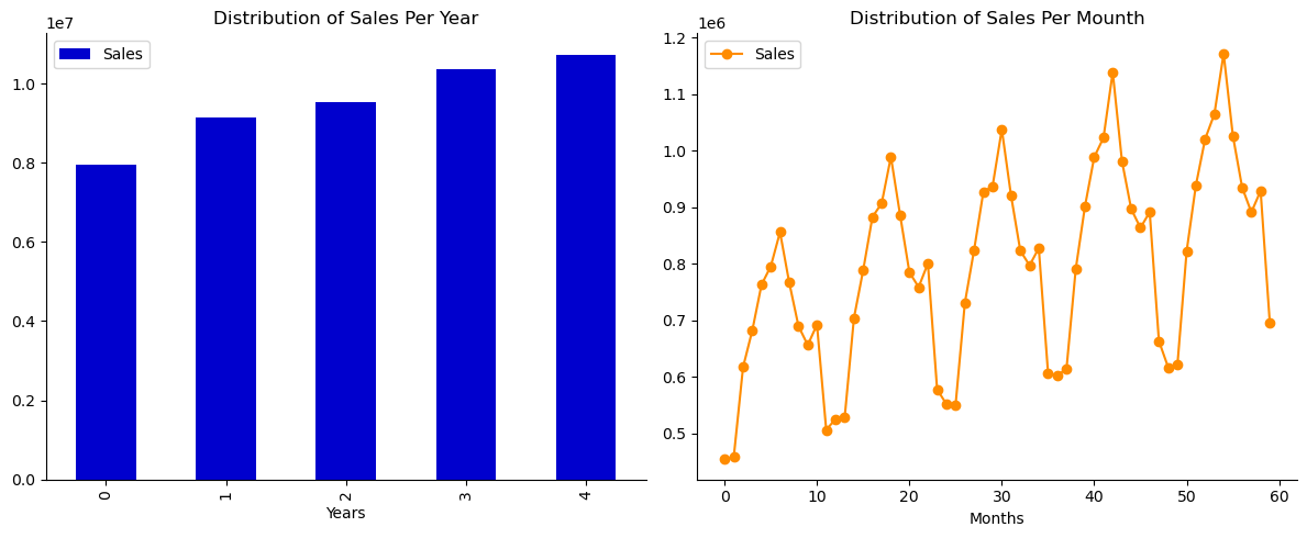

Note:

A number of alternative models, including weighted moving average models and autoregressive integrated moving average (ARIMA) models, can be used to forecast time series. Some of them need the trend and seasonality removed first. For instance, you would have to exclude this trend from the time series if you were analyzing the number of active visitors on your website, and it was increasing by 10% each month. To obtain the final forecasts, you would need to add the trend back after the model has been trained and has begun to make predictions. Similarly to this, if you were attempting to forecast the monthly sales of sunscreen lotion, you would likely see considerable seasonality: since it sells well during the summer, the same pattern would be repeated every year.

By computing the difference between the value at each time step and the value from one year earlier, for instance, you would be able to eliminate this seasonality from the time series (this technique is called differencing). Again, to obtain the final forecasts, you would need to re-add the seasonal pattern once the model has been trained and has made several predictions.

3. EDA(Exploratory Data Analysis)

We will compute the difference between each month's sales and add it as a new column to our data frame to make it stationary.

The sales_time() function will print the total time taken for stores in days, years and months.

Output: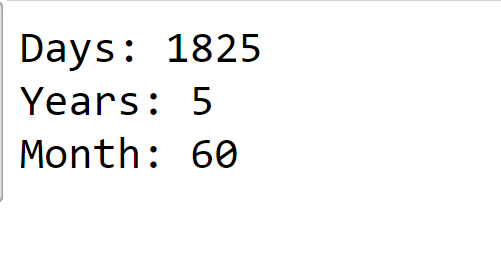

The above function represents the sales in each store.

Output: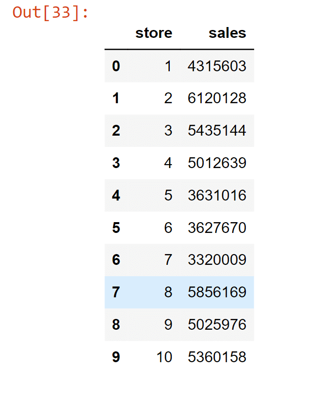

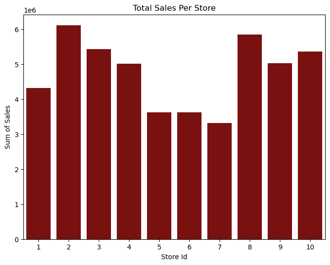
The above graph represents the total sale from each store.

From the above graph, we can interpret that Store Id 2 has the highest sales of 6120128 and the lowest sales is Store Id 7 of 5856169.

Output: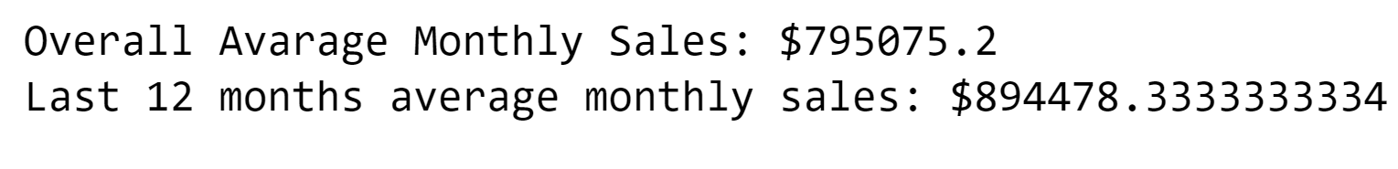

4. Determining Time Series Stationary

The fundamental idea is to simulate or estimate the trend and seasonality present in the series and then subtract these to get a stationary series. Then, this series can use statistical forecasting techniques. By putting trend and seasonality restrictions back, the anticipated values would then be converted into the original scale.

Output: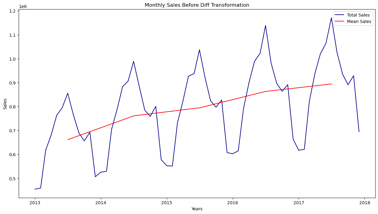

5. Differencing

We will calculate the difference between subsequent words in the series using this way. The changing mean is often eliminated using differencing.

Output: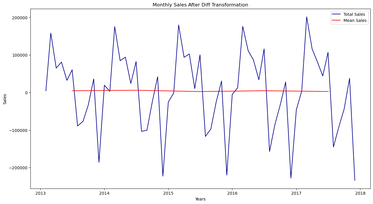

Now, we will set up the data for our various model types, that it represents monthly sales and has been modified to be stationary.

To do this, we'll define two distinct structures:

1. One is going to be used for ARIMA modelling.
2. The remaining models will utilize the other.

ARIMA Modeling

ARIMA (AutoRegressive Integrated Moving Average) is a popular time series forecasting model used for univariate time series data.

ARIMA models are fit to time series data to make predictions about future values. The process of fitting an ARIMA model involves selecting the order of the AR, I, and MA components, as well as the coefficients of each component. These coefficients are estimated using optimization algorithms like maximum likelihood estimation or numerical optimization. The resulting model can then be used to generate predictions for future values of the time series.

Output: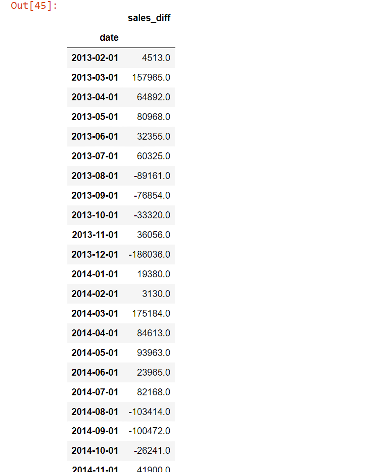

Observing Lags

Observing lags is an important step in the ARIMA modelling process. The goal of observing lags is to determine the order of the autoregressive (AR) component in the ARIMA model. The autoregressive component is based on past values of the time series, and the order of the AR component determines the number of past values that are used as predictors.

To observe lags, you typically plot the autocorrelation function (ACF) and partial autocorrelation function (PACF) of the time series. The ACF is a plot of the correlation between the time series and lagged versions of itself, while the PACF is a plot of the correlation between the time series and its lagged values, controlling for the effects of any intermediate lags.

To build a new data frame for our other models, we will assign each character to a prior month's sales. We will look at the autocorrelation and partial autocorrelation plots and use the guidelines for selecting lags in ARIMA modelling to decide how many months to include in our feature set. We can maintain a constant look-back time for both our ARIMA and regressive models in this way.

Output: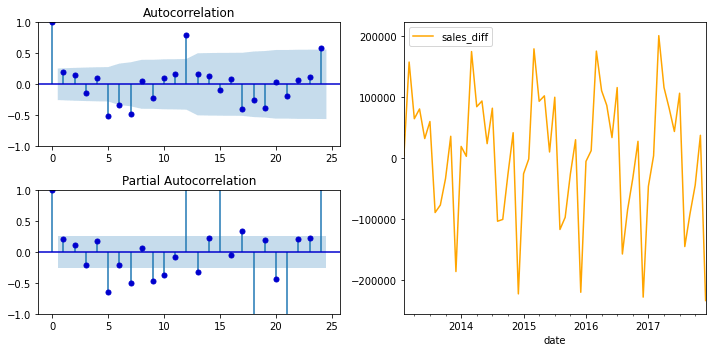

Regressive Modeling

Regression modelling is a statistical method used to model the relationship between a dependent variable and one or more independent variables. The goal of regression modelling is to identify the relationship between the independent variables and the dependent variable and to use this relationship to make predictions about the dependent variable.

Let's make a CSV file with columns for sales, dependent variables, and prior sales for each delay, and rows for each month. The EDA is used to construct the 12 delay characteristics. Regression modelling uses data.

Output: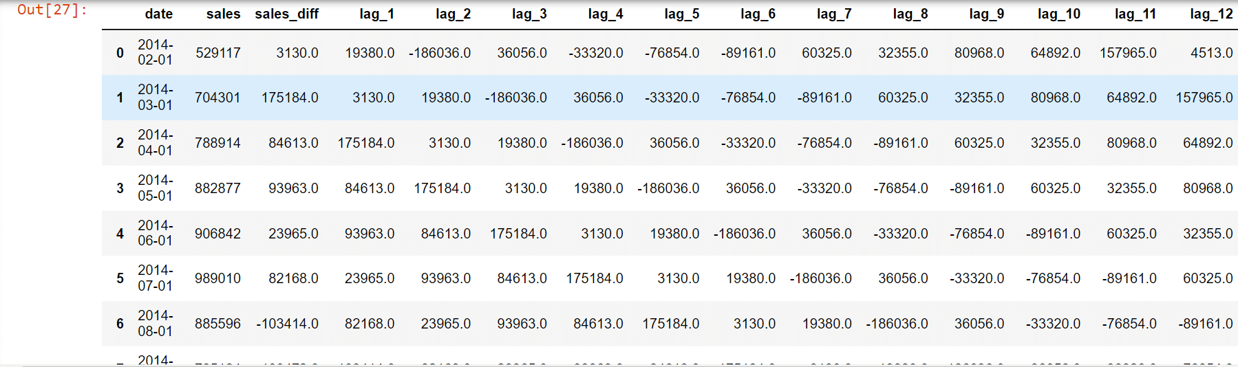

Output: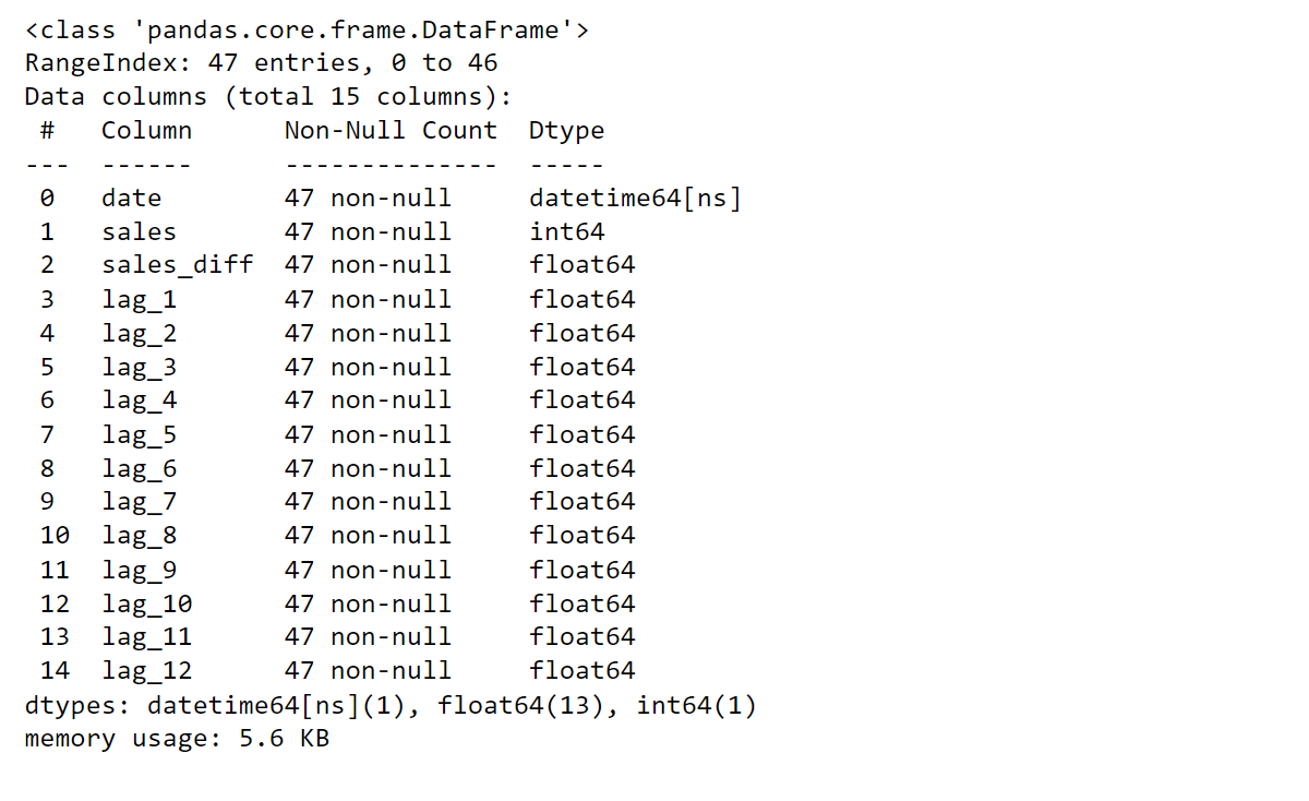

We detach our data so that the last 12 months are part of the test set, and the rest of the data is used to train our model.

Train and test Data

Output: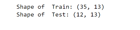

6. Scaling Data

Scaling data is the process of transforming the values of the variables in a dataset so that they are in a similar range. This is often done to prevent some variables from having an undue influence on the model due to their large scale.

Output: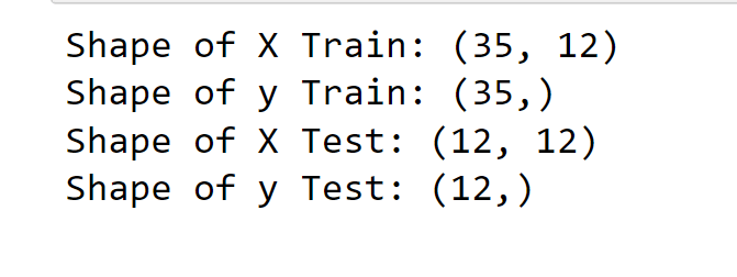

7. Reverse Scaling

Reverse scaling is the process of transforming a set of scaled variables back to their original scale. This can be necessary when you want to interpret the results of a modelling analysis in terms of the original variables rather than the scaled variables. The process of reverse scaling depends on the method used to scale the data.

We now have two distinct data structures:

• We have a DataTime index in our ARIMA structure.
• Lags are characteristics of our supervised structure.

8. Predictions DataFrame

Model Score

A model score function is a function that measures the accuracy or performance of a predictive model. The score function provides a quantitative measure of the model's ability to make accurate predictions, and it is used to compare different models and select the best model for a particular task.

This helper function will save the root mean squared error (RMSE) and mean absolute error (MAE) of our predictions to compare the performance of our models.

Graph

With this plot_results() function, it will plot a line graph of the model.

Modelling

We will use the underlying regression model for our task:

• Linear Regression
• Random Forest Regressor
• XGBoost
• LSTM

Now we will try to find the RMSE, MAE and R2 Score through each model.

1. Linear Regression

Linear Regression is a statistical method used for modelling the linear relationship between a dependent variable and one or more independent variables. It is a type of supervised learning, which means that it is used for making predictions based on input variables.

Output: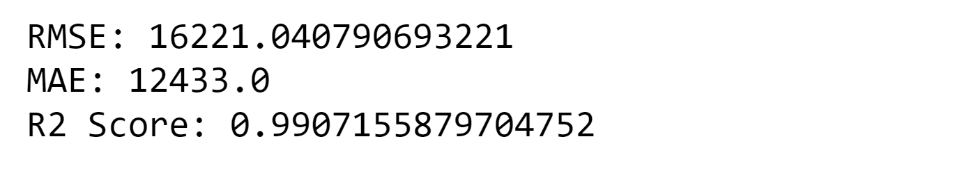

Random Forest Regressor

Random Forest Regressor is a type of ensemble learning method used for regression problems. It is an extension of the decision tree algorithm, where multiple decision trees are combined to form a forest.

Output: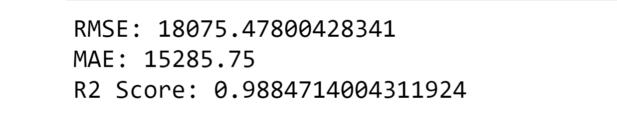

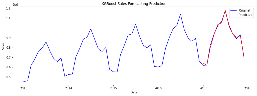
3. XGBOOST

XGBoost Regression is a specific implementation of the XGBoost algorithm for regression problems, where the goal is to predict a continuous target variable. It can handle both linear and non-linear relationships between the independent and dependent variables, as well as handle large datasets and missing data.

Output: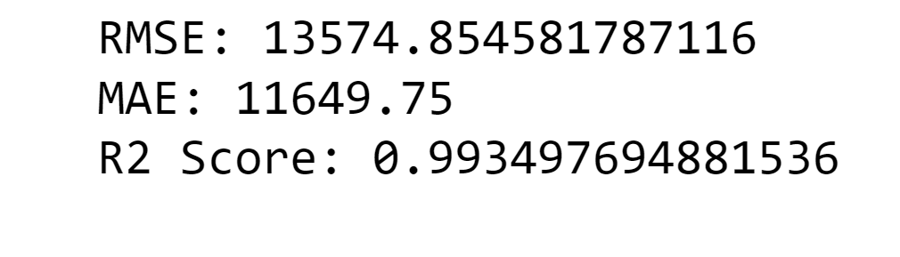

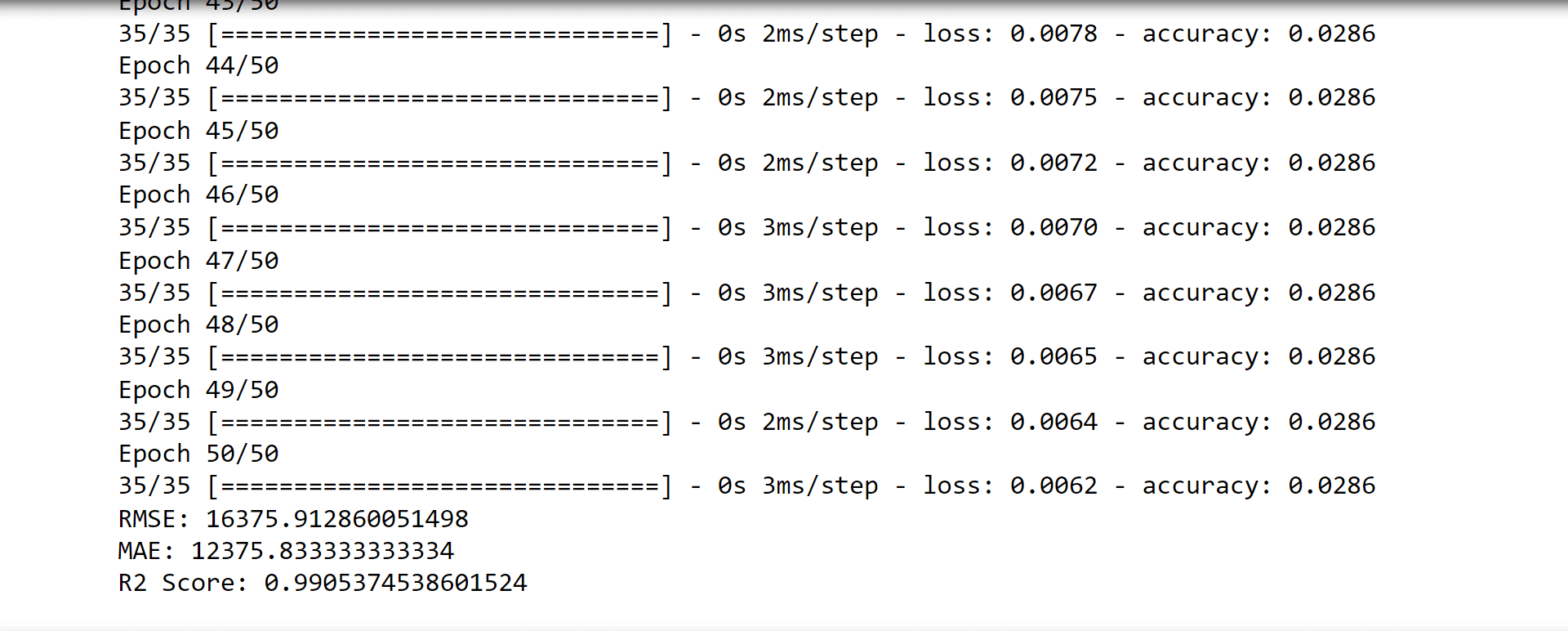
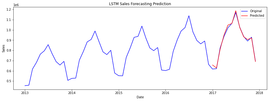
LSTM

LSTM is a type of recurrent neural network that is especially useful for predicting sequential data.

Output: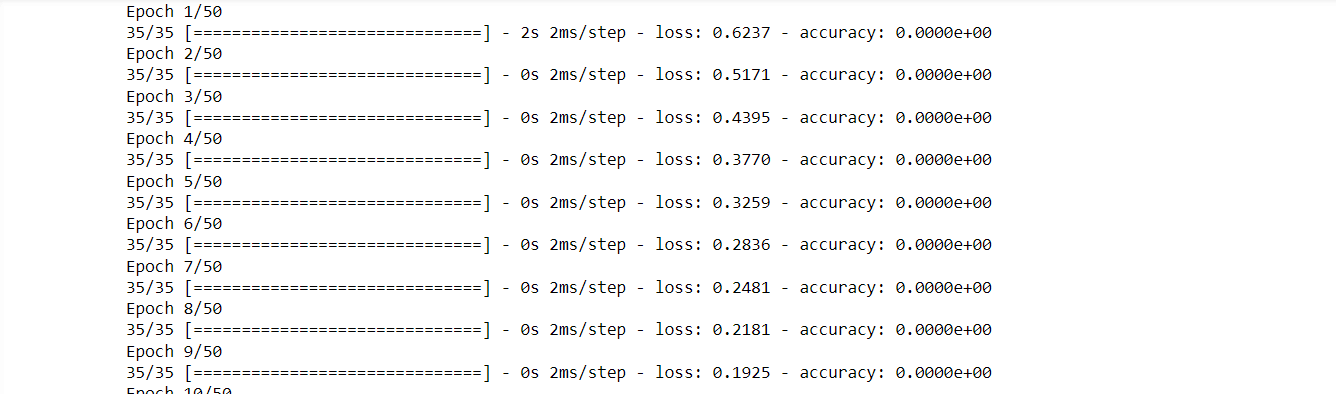

ARIMA MODELING

Output: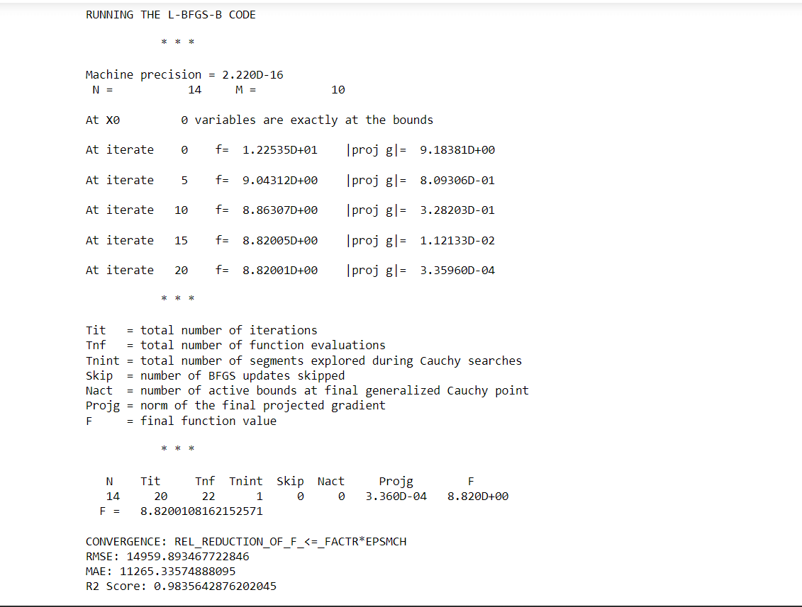

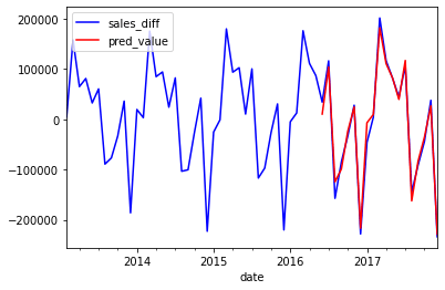
Output: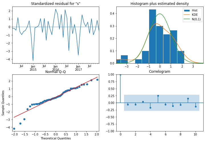

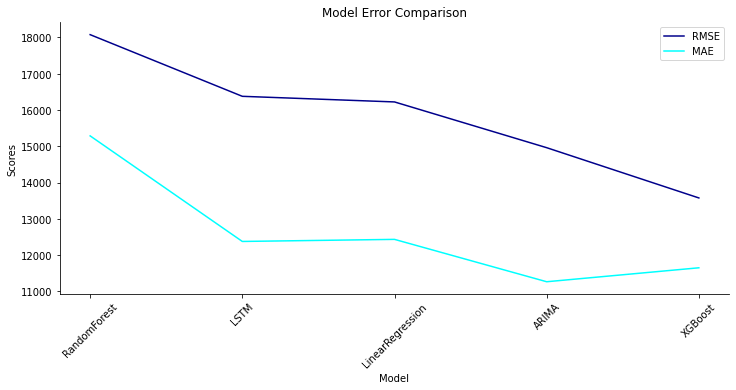
Compare Model

Comparing different machine learning models is an important step in the process of building a predictive model. When comparing models, several factors should be considered, that includes; Accuracy, Training time, Scalability, Model Complexity, Overfitting, Interpretability, Flexibility, Prediction time etc.

But in our case, we will consider the RMSE, MAE and R2 Score.

Output: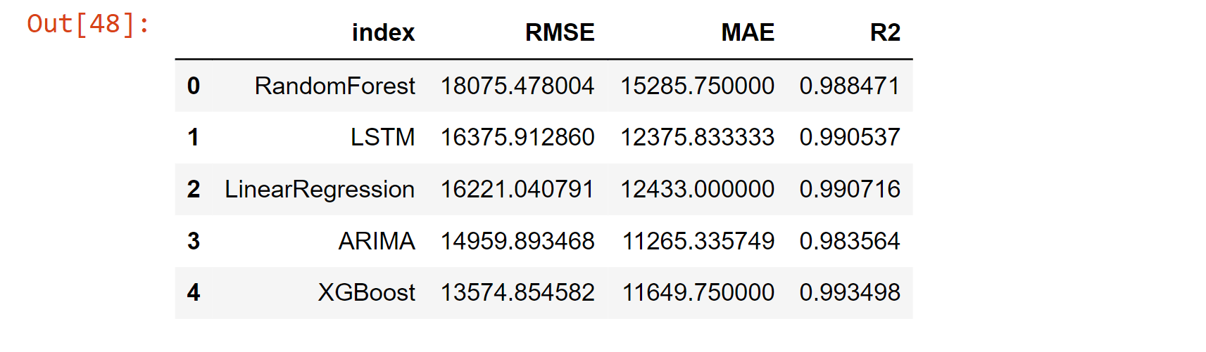

Output:

Output:

While comparing the model, we find that XGBoost has the lowest RMSE Score of 13574.854582, which concludes that it has the highest accuracy among the other models.

Through the percentage_off test, we find that XGBoost has the predictions that are actually in the percentage of 1.3% considering the actual prediction.

Overall, machine learning can be a powerful tool for predicting sales and improving business outcomes. Whether you are using regression analysis, time series analysis, decision tree-based algorithms or neural networks, machine learning can help you make more accurate predictions and take action to improve your sales.

Note: It's important to note that, as with any predictive model, the accuracy of the predictions will depend on the quality and quantity of data used to train the model. Therefore, it's essential to have a good understanding of the data and the underlying business problem in order to design a good model.

Conclusion

In conclusion, Machine Learning can be a powerful tool in the hands of businesses to predict sales and make informed decisions. With a combination of various algorithms, historical data and neural networks, businesses can improve their sales and make better decisions for their future.