Multiple Linear Regression

In the previous topic, we have learned about Simple Linear Regression, where a single Independent/Predictor(X) variable is used to model the response variable (Y). But there may be various cases in which the response variable is affected by more than one predictor variable; for such cases, the Multiple Linear Regression algorithm is used.

Moreover, Multiple Linear Regression is an extension of Simple Linear regression as it takes more than one predictor variable to predict the response variable. We can define it as:

Multiple Linear Regression is one of the important regression algorithms which models the linear relationship between a single dependent continuous variable and more than one independent variable.

Example:

Prediction of CO₂ emission based on engine size and number of cylinders in a car.

Some key points about MLR:

• For MLR, the dependent or target variable(Y) must be the continuous/real, but the predictor or independent variable may be of continuous or categorical form.
• Each feature variable must model the linear relationship with the dependent variable.
• MLR tries to fit a regression line through a multidimensional space of data-points.

MLR equation:

In Multiple Linear Regression, the target variable(Y) is a linear combination of multiple predictor variables x₁, x₂, x₃, ...,x_n. Since it is an enhancement of Simple Linear Regression, so the same is applied for the multiple linear regression equation, the equation becomes:

Where,

Y= Output/Response variable

b₀, b₁, b₂, b₃ , b_n....= Coefficients of the model.

x₁, x₂, x₃, x₄,...= Various Independent/feature variable

Assumptions for Multiple Linear Regression:

• A linear relationship should exist between the Target and predictor variables.
• The regression residuals must be normally distributed.
• MLR assumes little or no multicollinearity (correlation between the independent variable) in data.

Implementation of Multiple Linear Regression model using Python:

To implement MLR using Python, we have below problem:

Problem Description:

We have a dataset of 50 start-up companies. This dataset contains five main information: R&D Spend, Administration Spend, Marketing Spend, State, and Profit for a financial year. Our goal is to create a model that can easily determine which company has a maximum profit, and which is the most affecting factor for the profit of a company.

Since we need to find the Profit, so it is the dependent variable, and the other four variables are independent variables. Below are the main steps of deploying the MLR model:

1. Data Pre-processing Steps
2. Fitting the MLR model to the training set
3. Predicting the result of the test set

Step-1: Data Pre-processing Step:

The very first step is data pre-processing, which we have already discussed in this tutorial. This process contains the below steps:

• Importing libraries: Firstly we will import the library which will help in building the model. Below is the code for it:

• Importing dataset: Now we will import the dataset(50_CompList), which contains all the variables. Below is the code for it:

Output: We will get the dataset as: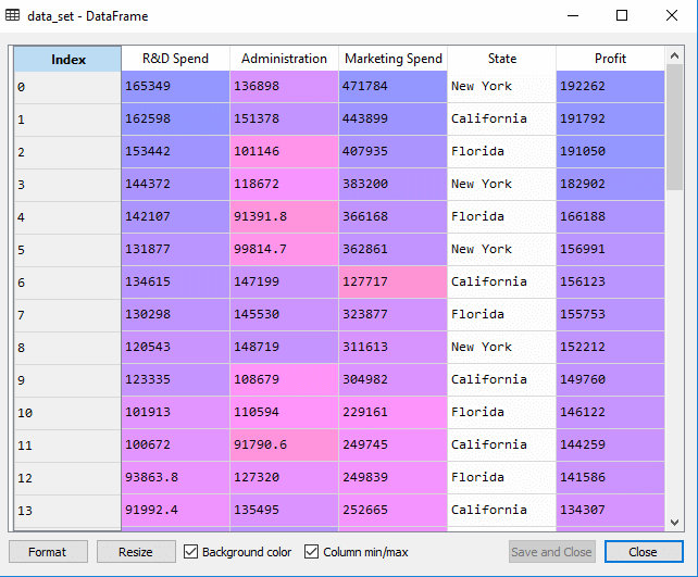

In above output, we can clearly see that there are five variables, in which four variables are continuous and one is categorical variable.

• Extracting dependent and independent Variables:

Output:

Out[5]:

array([[165349.2, 136897.8, 471784.1, 'New York'],
       [162597.7, 151377.59, 443898.53, 'California'],
       [153441.51, 101145.55, 407934.54, 'Florida'],
       [144372.41, 118671.85, 383199.62, 'New York'],
       [142107.34, 91391.77, 366168.42, 'Florida'],
       [131876.9, 99814.71, 362861.36, 'New York'],
       [134615.46, 147198.87, 127716.82, 'California'],
       [130298.13, 145530.06, 323876.68, 'Florida'],
       [120542.52, 148718.95, 311613.29, 'New York'],
       [123334.88, 108679.17, 304981.62, 'California'],
       [101913.08, 110594.11, 229160.95, 'Florida'],
       [100671.96, 91790.61, 249744.55, 'California'],
       [93863.75, 127320.38, 249839.44, 'Florida'],
       [91992.39, 135495.07, 252664.93, 'California'],
       [119943.24, 156547.42, 256512.92, 'Florida'],
       [114523.61, 122616.84, 261776.23, 'New York'],
       [78013.11, 121597.55, 264346.06, 'California'],
       [94657.16, 145077.58, 282574.31, 'New York'],
       [91749.16, 114175.79, 294919.57, 'Florida'],
       [86419.7, 153514.11, 0.0, 'New York'],
       [76253.86, 113867.3, 298664.47, 'California'],
       [78389.47, 153773.43, 299737.29, 'New York'],
       [73994.56, 122782.75, 303319.26, 'Florida'],
       [67532.53, 105751.03, 304768.73, 'Florida'],
       [77044.01, 99281.34, 140574.81, 'New York'],
       [64664.71, 139553.16, 137962.62, 'California'],
       [75328.87, 144135.98, 134050.07, 'Florida'],
       [72107.6, 127864.55, 353183.81, 'New York'],
       [66051.52, 182645.56, 118148.2, 'Florida'],
       [65605.48, 153032.06, 107138.38, 'New York'],
       [61994.48, 115641.28, 91131.24, 'Florida'],
       [61136.38, 152701.92, 88218.23, 'New York'],
       [63408.86, 129219.61, 46085.25, 'California'],
       [55493.95, 103057.49, 214634.81, 'Florida'],
       [46426.07, 157693.92, 210797.67, 'California'],
       [46014.02, 85047.44, 205517.64, 'New York'],
       [28663.76, 127056.21, 201126.82, 'Florida'],
       [44069.95, 51283.14, 197029.42, 'California'],
       [20229.59, 65947.93, 185265.1, 'New York'],
       [38558.51, 82982.09, 174999.3, 'California'],
       [28754.33, 118546.05, 172795.67, 'California'],
       [27892.92, 84710.77, 164470.71, 'Florida'],
       [23640.93, 96189.63, 148001.11, 'California'],
       [15505.73, 127382.3, 35534.17, 'New York'],
       [22177.74, 154806.14, 28334.72, 'California'],
       [1000.23, 124153.04, 1903.93, 'New York'],
       [1315.46, 115816.21, 297114.46, 'Florida'],
       [0.0, 135426.92, 0.0, 'California'],
       [542.05, 51743.15, 0.0, 'New York'],
       [0.0, 116983.8, 45173.06, 'California']], dtype=object)

As we can see in the above output, the last column contains categorical variables which are not suitable to apply directly for fitting the model. So we need to encode this variable.

Encoding Dummy Variables:

As we have one categorical variable (State), which cannot be directly applied to the model, so we will encode it. To encode the categorical variable into numbers, we will use the LabelEncoder class. But it is not sufficient because it still has some relational order, which may create a wrong model. So in order to remove this problem, we will use OneHotEncoder, which will create the dummy variables. Below is code for it:

Here we are only encoding one independent variable, which is state as other variables are continuous.

Output: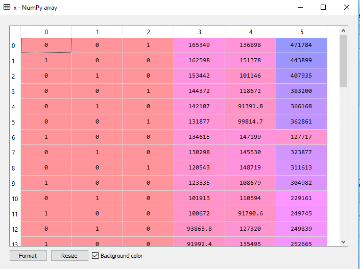

As we can see in the above output, the state column has been converted into dummy variables (0 and 1). Here each dummy variable column is corresponding to the one State. We can check by comparing it with the original dataset. The first column corresponds to the California State, the second column corresponds to the Florida State, and the third column corresponds to the New York State.

Note: We should not use all the dummy variables at the same time, so it must be 1 less than the total number of dummy variables, else it will create a dummy variable trap.

• Now, we are writing a single line of code just to avoid the dummy variable trap:

If we do not remove the first dummy variable, then it may introduce multicollinearity in the model.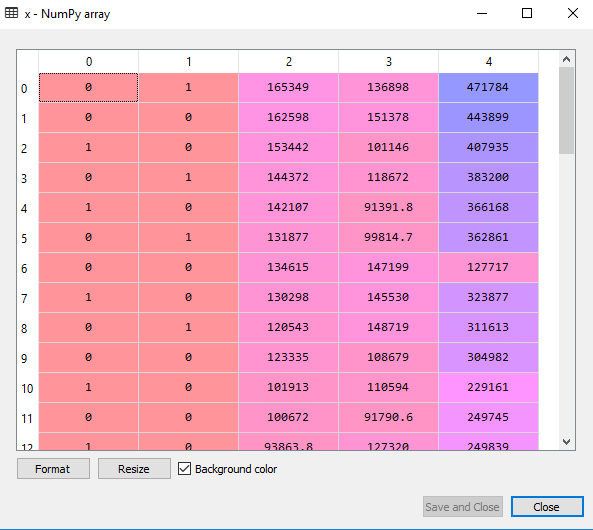

As we can see in the above output image, the first column has been removed.

• Now we will split the dataset into training and test set. The code for this is given below:

The above code will split our dataset into a training set and test set.

Output: The above code will split the dataset into training set and test set. You can check the output by clicking on the variable explorer option given in Spyder IDE. The test set and training set will look like the below image:

Test set: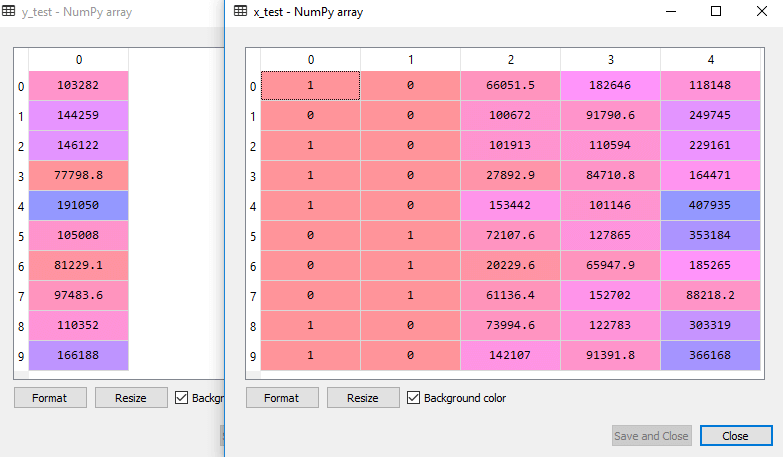

Training set: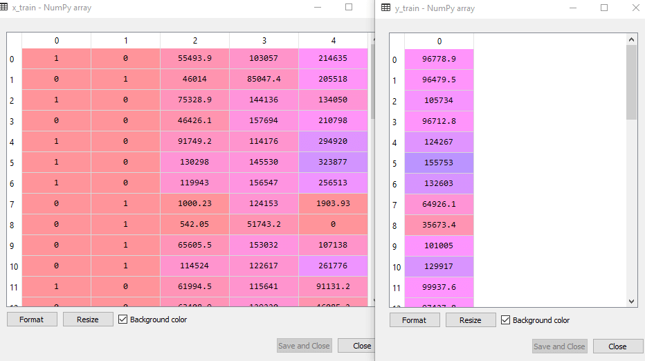

Note: In MLR, we will not do feature scaling as it is taken care by the library, so we don't need to do it manually.

Step: 2- Fitting our MLR model to the Training set:

Now, we have well prepared our dataset in order to provide training, which means we will fit our regression model to the training set. It will be similar to as we did in Simple Linear Regression model. The code for this will be:

Output:

Out[9]: LinearRegression(copy_X=True, fit_intercept=True, n_jobs=None, normalize=False)

Now, we have successfully trained our model using the training dataset. In the next step, we will test the performance of the model using the test dataset.

Step: 3- Prediction of Test set results:

The last step for our model is checking the performance of the model. We will do it by predicting the test set result. For prediction, we will create a y_pred vector. Below is the code for it:

By executing the above lines of code, a new vector will be generated under the variable explorer option. We can test our model by comparing the predicted values and test set values.

Output: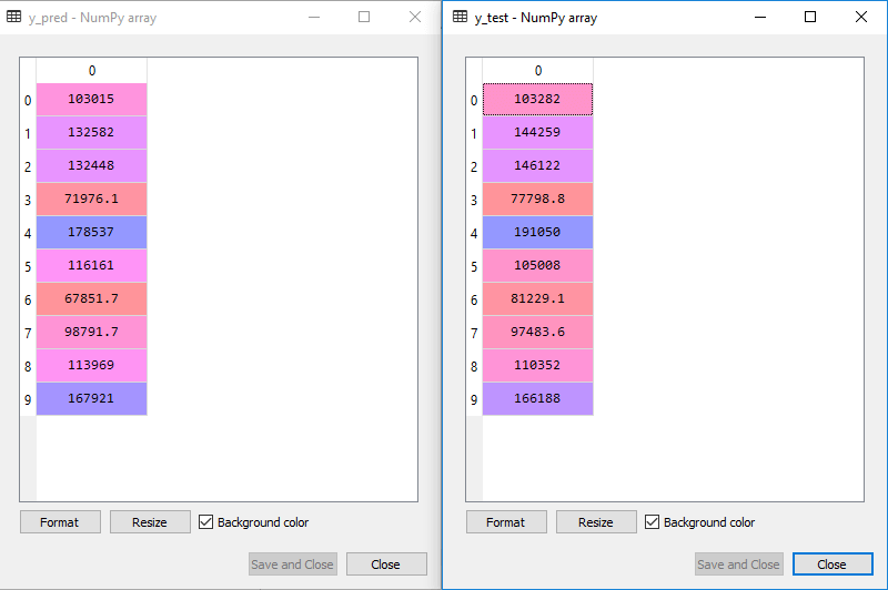

In the above output, we have predicted result set and test set. We can check model performance by comparing these two value index by index. For example, the first index has a predicted value of 103015$ profit and test/real value of 103282$ profit. The difference is only of 267$, which is a good prediction, so, finally, our model is completed here.

• We can also check the score for training dataset and test dataset. Below is the code for it:

Output: The score is:

Train Score:  0.9501847627493607
Test Score:  0.9347068473282446

The above score tells that our model is 95% accurate with the training dataset and 93% accurate with the test dataset.

Note: In the next topic, we will see how we can improve the performance of the model using the Backward Elimination process.

Applications of Multiple Linear Regression:

There are mainly two applications of Multiple Linear Regression:

• Effectiveness of Independent variable on prediction:
• Predicting the impact of changes: