GBM in Machine Learning

Machine learning is one of the most popular technologies to build predictive models for various complex regression and classification tasks. Gradient Boosting Machine (GBM) is considered one of the most powerful boosting algorithms.

Although, there are so many algorithms used in machine learning, boosting algorithms has become mainstream in the machine learning community across the world. Boosting technique follows the concept of ensemble learning, and hence it combines multiple simple models (weak learners or base estimators) to generate the final output. GBM is also used as an ensemble method in machine learning which converts the weak learners into strong learners. In this topic, "GBM in Machine Learning" we will discuss gradient machine learning algorithms, various boosting algorithms in machine learning, the history of GBM, how it works, various terminologies used in GBM, etc. But before starting, first, understand the boosting concept and various boosting algorithms in machine learning.

What is Boosting in Machine Learning?

Boosting is one of the popular learning ensemble modeling techniques used to build strong classifiers from various weak classifiers. It starts with building a primary model from available training data sets then it identifies the errors present in the base model. After identifying the error, a secondary model is built, and further, a third model is introduced in this process. In this way, this process of introducing more models is continued until we get a complete training data set by which model predicts correctly.

AdaBoost (Adaptive boosting) was the first boosting algorithm to combine various weak classifiers into a single strong classifier in the history of machine learning. It primarily focuses to solve classification tasks such as binary classification.

Steps in Boosting Algorithms:

There are a few important steps in boosting the algorithm as follows:

• Consider a dataset having different data points and initialize it.
• Now, give equal weight to each of the data points.
• Assume this weight as an input for the model.
• Identify the data points that are incorrectly classified.
• Increase the weight for data points in step 4.
• If you get appropriate output then terminate this process else follow steps 2 and 3 again.

Example:

Let's suppose, we have three different models with their predictions and they work in completely different ways. For example, the linear regression model shows a linear relationship in data while the decision tree model attempts to capture the non-linearity in the data as shown below image.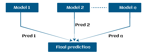

Further, instead of using these models separately to predict the outcome if we use them in form of series or combination, then we get a resulting model with correct information than all base models. In other words, instead of using each model's individual prediction, if we use average prediction from these models then we would be able to capture more information from the data. It is referred to as ensemble learning and boosting is also based on ensemble methods in machine learning.

Boosting Algorithms in Machine Learning

There are primarily 4 boosting algorithms in machine learning. These are as follows:

• Gradient Boosting Machine (GBM)
• Extreme Gradient Boosting Machine (XGBM)
• Light GBM
• CatBoost

What is GBM in Machine Learning?

Gradient Boosting Machine (GBM) is one of the most popular forward learning ensemble methods in machine learning. It is a powerful technique for building predictive models for regression and classification tasks.

GBM helps us to get a predictive model in form of an ensemble of weak prediction models such as decision trees. Whenever a decision tree performs as a weak learner then the resulting algorithm is called gradient-boosted trees.

It enables us to combine the predictions from various learner models and build a final predictive model having the correct prediction.

But here one question may arise if we are applying the same algorithm then how multiple decision trees can give better predictions than a single decision tree? Moreover, how does each decision tree capture different information from the same data?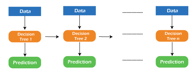

So, the answer to these questions is that a different subset of features is taken by the nodes of each decision tree to select the best split. It means, that each tree behaves differently, and hence captures different signals from the same data.

How do GBM works?

Generally, most supervised learning algorithms are based on a single predictive model such as linear regression, penalized regression model, decision trees, etc. But there are some supervised algorithms in ML that depend on a combination of various models together through the ensemble. In other words, when multiple base models contribute their predictions, an average of all predictions is adapted by boosting algorithms.

Gradient boosting machines consist 3 elements as follows:

• Loss function
• Weak learners
• Additive model

Let's understand these three elements in detail.

1. Loss function:

Although, there is a big family of Loss functions in machine learning that can be used depending on the type of tasks being solved. The use of the loss function is estimated by the demand of specific characteristics of the conditional distribution such as robustness. While using a loss function in our task, we must specify the loss function and the function to calculate the corresponding negative gradient. Once, we get these two functions, they can be implemented into gradient boosting machines easily. However, there are several loss functions have been already proposed for GBM algorithms.

Classification of loss function:

Based on the type of response variable y, loss function can be classified into different types as follows:

1. Continuous response, y ∈ R:
   • Gaussian L2 loss function
   • Laplace L1 loss function
   • Huber loss function, δ specified
   • Quantile loss function, α specified
2. Categorical response, y ∈ {0, 1}:
   • Binomial loss function
   • Adaboost loss function
3. Other families of response variables:
   • Loss functions for survival models
   • Loss functions count data
   • Custom loss functions

2. Weak Learner:

Weak learners are the base learner models that learn from past errors and help in building a strong predictive model design for boosting algorithms in machine learning. Generally, decision trees work as a weak learners in boosting algorithms.

Boosting is defined as the framework that continuously works to improve the output from base models. Many gradient boosting applications allow you to "plugin" various classes of weak learners at your disposal. Hence, decision trees are most often used for weak (base) learners.

How to train weak learners:

Machine learning uses training datasets to train base learners and based on the prediction from the previous learner, it improves the performance by focusing on the rows of the training data where the previous tree had the largest errors or residuals. E.g. shallow trees are considered weak learner to decision trees as it contains a few splits. Generally, in boosting algorithms, trees having up to 6 splits are most common.

Below is a sequence of training the weak learner to improve their performance where each tree is in the sequence with the previous tree's residuals. Further, we are introducing each new tree so that it can learn from the previous tree's errors. These are as follows:

1. Consider a data set and fit a decision tree into it.
   F1(x)=y
2. Fit the next decision tree with the largest errors of the previous tree.
   h1(x)=y?F1(x)
3. Add this new tree to the algorithm by adding both in steps 1 and 2.
   F2(x)=F1(x)+h1(x)
4. Again fit the next decision tree with the residuals of the previous tree.
   h2(x)=y?F2(x)
5. Repeat the same which we have done in step 3.
   F3(x)=F2(x)+h2(x)

Continue this process until some mechanism (i.e. cross-validation) tells us to stop. The final model here is a stagewise additive model of b individual trees:

Hence, trees are constructed greedily, choosing the best split points based on purity scores like Gini or minimizing the loss.

3. Additive Model:

The additive model is defined as adding trees to the model. Although we should not add multiple trees at a time, only a single tree must be added so that existing trees in the model are not changed. Further, we can also prefer the gradient descent method by adding trees to reduce the loss.

In the past few years, the gradient descent method was used to minimize the set of parameters such as the coefficient of the regression equation and weight in a neural network. After calculating error or loss, the weight parameter is used to minimize the error. But recently, most ML experts prefer weak learner sub-models or decision trees as a substitute for these parameters. In which, we have to add a tree in the model to reduce the error and improve the performance of that model. In this way, the prediction from the newly added tree is combined with the prediction from the existing series of trees to get a final prediction. This process continues until the loss reaches an acceptable level or is no longer improvement required.

This method is also known as functional gradient descent or gradient descent with functions.

EXTREME GRADIENT BOOSTING MACHINE (XGBM)

XGBM is the latest version of gradient boosting machines which also works very similar to GBM. In XGBM, trees are added sequentially (one at a time) that learn from the errors of previous trees and improve them. Although, XGBM and GBM algorithms are similar in look and feel but still there are a few differences between them as follows:

• XGBM uses various regularization techniques to reduce under-fitting or over-fitting of the model which also increases model performance more than gradient boosting machines.
• XGBM follows parallel processing of each node, while GBM does not which makes it more rapid than gradient boosting machines.
• XGBM helps us to get rid of the imputation of missing values because by default the model takes care of it. It learns on its own whether these values should be in the right or left node.

Light Gradient Boosting Machines (Light GBM)

Light GBM is a more upgraded version of the Gradient boosting machine due to its efficiency and fast speed. Unlike GBM and XGBM, it can handle a huge amount of data without any complexity. On the other hand, it is not suitable for those data points that are lesser in number.

Instead of level-wise growth, Light GBM prefers leaf-wise growth of the nodes of the tree. Further, in light GBM, the primary node is split into two secondary nodes and later it chooses one secondary node to be split. This split of a secondary node depends upon which between two nodes has a higher loss.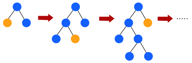

Hence, due to leaf-wise split, Light Gradient Boosting Machine (LGBM) algorithm is always preferred over others where a large amount of data is given.

CATBOOST

The catboost algorithm is primarily used to handle the categorical features in a dataset. Although GBM, XGBM, and Light GBM algorithms are suitable for numeric data sets, Catboost is designed to handle categorical variables into numeric data. Hence, catboost algorithm consists of an essential preprocessing step to convert categorical features into numerical variables which are not present in any other algorithm.

Advantages of Boosting Algorithms:

• Boosting algorithms follow ensemble learning which enables a model to give a more accurate prediction that cannot be trumped.
• Boosting algorithms are much more flexible than other algorithms as can optimize different loss functions and provides several hyperparameter tuning options.
• It does not require data pre-processing because it is suitable for both numeric as well as categorical variables.
• It does not require imputation of missing values in the dataset, it handles missing data automatically.

Disadvantages of Boosting Algorithms:

Below are a few disadvantages of boosting algorithms:

• Boosting algorithms may cause overfitting as well as overemphasizing the outliers.
• Gradient boosting algorithm continuously focuses to minimize the errors and requires multiple trees hence, it is computationally expensive.
• It is a time-consuming and memory exhaustive algorithm.
• Less interpretative in nature, although this is easily addressed with various tools.

Conclusion:

In this way, we have learned boosting algorithms for predictive modeling in machine learning. Also, we have discussed various important boosting algorithms used in ML such as GBM, XGBM, light GBM, and Catboost. Further, we have seen various components (loss function, weak learner, and additive model) and how GBM works with them. How boosting algorithms are advantageous for deployment in real-world scenarios, etc.