Image Processing Using Machine Learning

Image processing involves manipulating and analyzing images to enhance their quality, extract features, or recognize patterns. Traditional image processing techniques rely on predefined rules and algorithms to perform specific tasks, such as edge detection, image segmentation, or object recognition. However, these techniques often face limitations when dealing with complex and diverse visual data.

Machine learning, on the other hand, offers a more flexible and adaptive approach to image processing. By training algorithms on large datasets of labelled images, machine learning models can learn to recognize patterns and extract relevant features automatically. This ability to learn from data and adapt to new situations makes machine learning a powerful tool for image analysis and processing.

One of the key applications of machine learning in image processing is object detection and recognition. By training models on labelled images that contain objects of interest, such as cars, people, or buildings, machine learning algorithms can learn to identify and locate these objects in new images. This capability has significant implications in fields like surveillance, where automated object detection can assist in identifying potential threats or anomalies.

Another application of machine learning in image processing is image classification. By training models on labelled images from different categories, such as animals, landscapes, or medical images, machine learning algorithms can learn to classify new images into the appropriate categories. This capability is particularly useful in areas like healthcare, where accurate and automated image classification can aid in disease diagnosis, medical imaging analysis, and treatment planning.

Now for the sake of understanding, we will try to implement it. Here we will do image processing for nucleus detection.

Code:

Importing Libraries

#Importing the other necessary libraries
import numpy as np
import pandas as pd
import os
import pathlib
import seaborn as sns
import matplotlib.pyplot as plt
%matplotlib inline
import warnings
warnings.filterwarnings('ignore')
import cv2

Reading the Image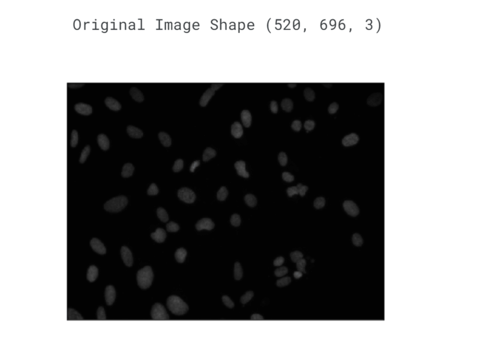

# Glob the training data and load a single image path
training_paths = pathlib.Path('../input/stage1_train').glob('*/images/*.png')
training_sorted = sorted([x for x in training_paths])
im_path = training_sorted[45]

#To read the image 
bgrimg = cv2.imread(str(im_path))
plt.imshow(bgrimg)
plt.xticks([]) #To get rid of the x-ticks and y-ticks on the image axis
plt.yticks([])
print('Original Image Shape',bgrimg.shape)

Output:

#To see the structure of the image, let's display one row of the image matrix
print('The first row of the image matrix contains',len(bgrimg[1]),'pixels')
print(bgrimg[1])

Output: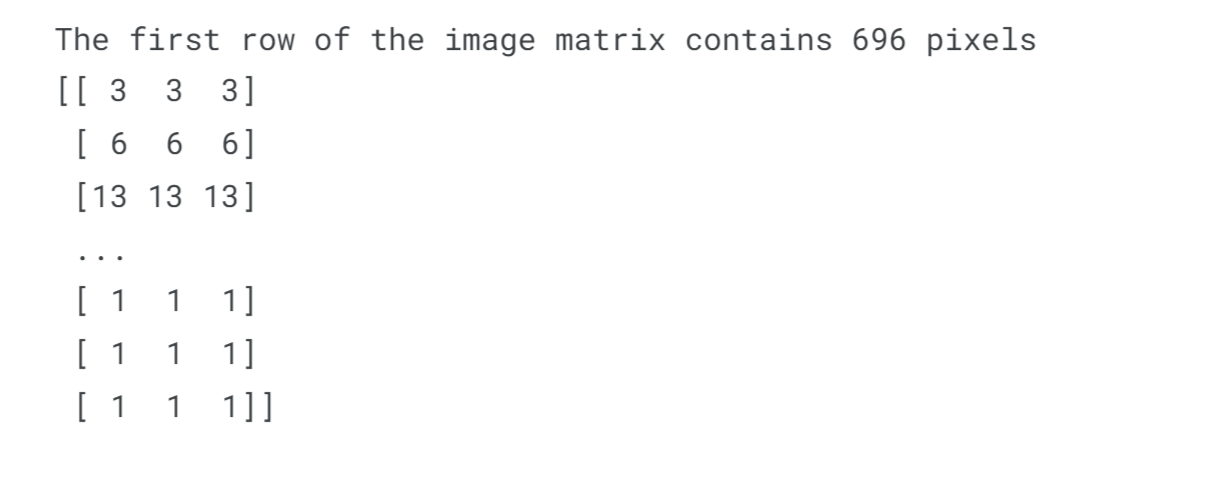

The image is being interpreted in the BGR (Blue-Green-Red) colourspace, which means that each pixel in the image is represented by three values: the intensity of blue, the intensity of green, and the intensity of red. This colourspace is the default choice when reading images in OpenCV.

In the BGR/RGB colourspace, specific combinations of red, green, and blue are used to create a wide range of colours. These three primary colours, when mixed together, can generate any chromaticity within the triangle formed by their respective values. In simpler terms, you can think of an RGB colour as encompassing all the possible colours that can be produced by mixing three coloured lights: red, green, and blue. By adjusting the intensity of these primary colours, we can create and display a vast array of different colours in an image.

Basic Steps

Here we will implement classical image techniques, which will hopefully serve as a useful primer.

Those classical image techniques are:

Dealing with Color
Removi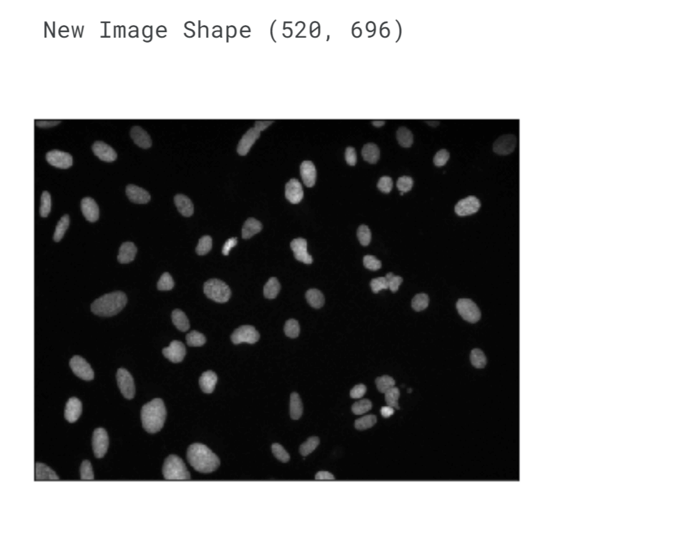ng Background
Deriving a Mask for each object
Object Identification
Run length encoding

Dealing with Color

#To transform the colourspace from BGR to grayscale so as to make things simpler
grayimg = cv2.cvtColor(bgrimg,cv2.COLOR_BGR2GRAY)

#To plot the image
plt.imshow(grayimg,cmap='gray') #cmap has been used as matplotlib uses some default colormap to plot grayscale images
plt.xticks([]) #To get rid of the x-ticks and y-ticks on the image axis
plt.yticks([])
print('New Image Shape',grayimg.shape)

Output:

When we converted the image from the BGR colourspace to grayscale, we actually reduced one dimension. This occurred because grayscale represents a range of monochromatic shades that go from black to white. In other words, a grayscale image only contains various shades of grey and lacks any colour information (it primarily consists of black and white).

The transformation from BGR to grayscale eliminates all colour data, retaining only the luminance of each pixel. In digital images, colours are displayed using a combination of red, green, and blue (RGB) values. Therefore, each pixel has three separate luminance values corresponding to these colour channels. However, when removing colour and creating a grayscale image, these three values need to be merged into a single value.

Luminance can also be described as brightness or intensity, which is measured on a scale ranging from black (zero intensity) to white (full intensity). By reducing the image to grayscale, we simplify its representation to focus solely on the variations in brightness across the image, disregarding the specific colours present.

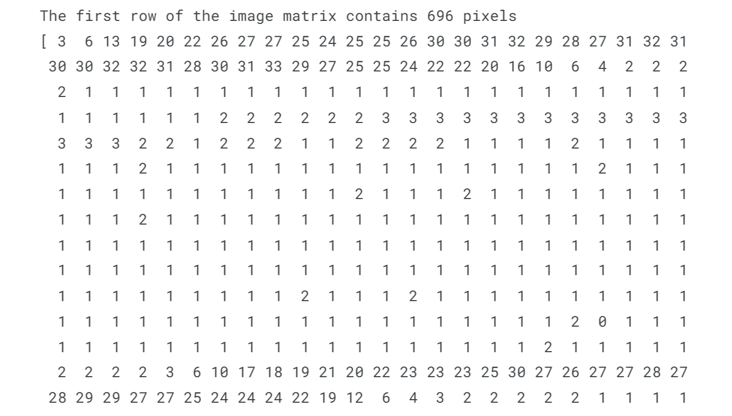
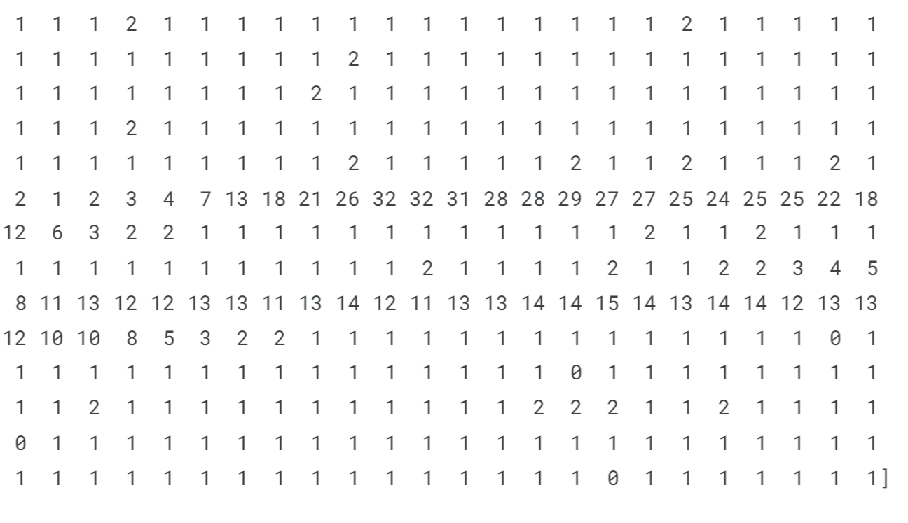
#To understand this further, let's display one entire row of the image matrix
print('The first row of the image matrix contains',len(grayimg[1]),'pixels')
print(grayimg[1])

Output:

When displaying one entire row of the image matrix in grayscale, you are essentially showing the luminance or intensity values of each pixel along that row. Each pixel's luminance value represents its brightness level, ranging from black (lowest intensity) to white (highest intensity).

By visualizing a row of the image matrix in grayscale, you can observe the varying intensities of the pixels within that row. This provides insight into the brightness patterns and transitions occurring horizontally across the image. It allows you to focus on the luminance variations without the distraction of colour information, highlighting the grayscale image's tonal values and emphasizing the contrast and shading present in that particular row.

Thus this displays one entire row of the image matrix with the corresponding luminance or intensities of every pixel.

Removing Background

#Okay, le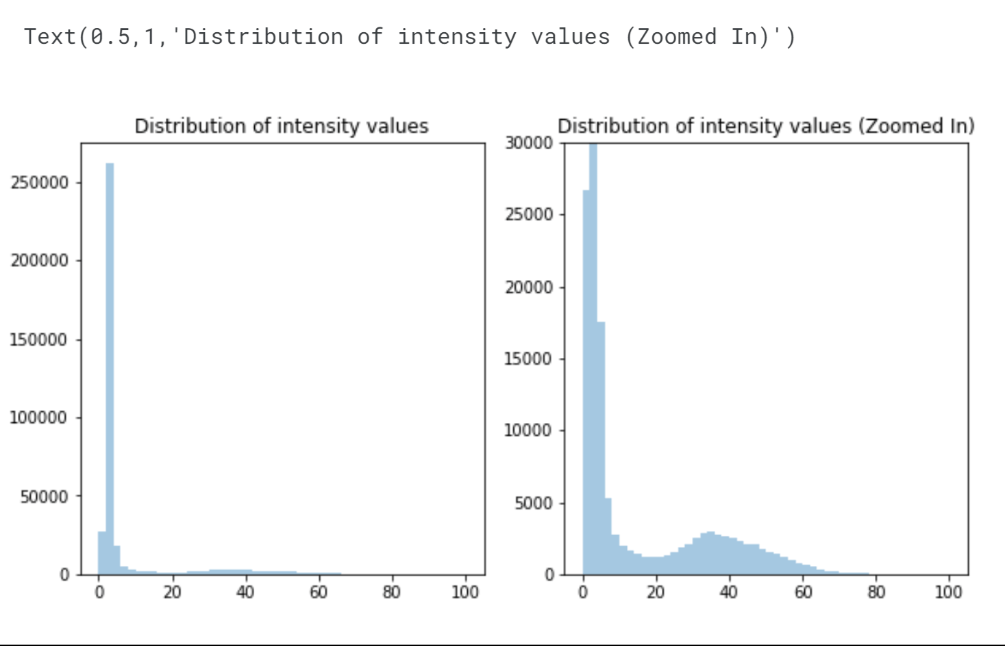t's look at the distribution of the intensity values of all the pixels
plt.figure(figsize=(10,5))

plt.subplot(1,2,1)
sns.distplot(grayimg.flatten(),kde=False)#This is to flatten the matrix and put the intensity values of all the pixels in one single row vector
plt.title('Distribution of intensity values')

#To zoom in on the distribution and see if there is more than one prominent peak 
plt.subplot(1,2,2)
sns.distplot(grayimg.flatten(),kde=False) 
plt.ylim(0,30000) 
plt.title('Distribution of intensity values (Zoomed In)')

Output:

We can observe two prominent peaks in the intensity distribution. The high count of pixels with intensity values around 0 is expected because the nuclei occupy a smaller portion of the image compared to the predominantly black background. Our task here is to separate the nuclei from the background. Based on the descriptive statistics, we anticipate an optimal separation value of approximately 20. However, instead of relying solely on such statistics, we should adopt a more formal approach like Otsu's method.

Otsu's method, named after Nobuyuki Otsu, is a technique used for automatic clustering-based image thresholding. It aims to convert a grayscale image into a binary image by identifying an optimal threshold. The algorithm assumes that the image consists of two classes of pixels, namely foreground pixels (nuclei) and background pixels. It calculates the threshold that minimizes the combined spread or intra-class variance of the two classes, thereby maximizing their inter-class variance. In simpler terms, Otsu's method determines the best threshold to separate the nuclei from the background based on the histogram distribution of pixel intensities.

from skimage.filters import threshold_otsu
thresh_val = threshold_otsu(grayimg)
print('The optimal seperation value is',thresh_val)

Output:

We will encode the pixels based on their intensity values using the np.where function, we can create a mask that sets all pixels with an intensity value greater than the threshold value to 1, and all other pixels to 0. The resulting mask will indicate the separation between the nuclei (encoded as 1) and the background (encoded as 0).

Deriving Mask for each object

mask=np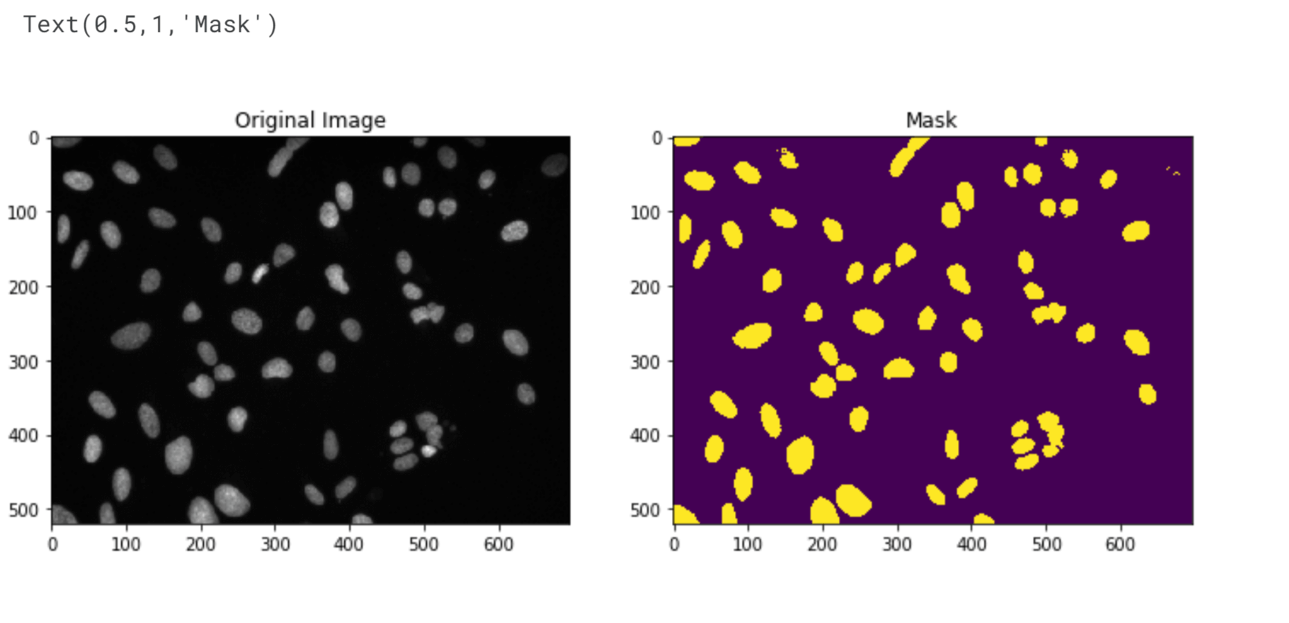.where(grayimg>thresh_val,1,0)

#To plot the original image and mask side by side
plt.figure(figsize=(12,6))
plt.subplot(1,2,1)
plt.imshow(grayimg,cmap='gray')
plt.title('Original Image')

plt.subplot(1,2,2)
maskimg = mask.copy()
plt.imshow(maskimg, cmap='viridis')
plt.title('Mask')

Output:

The current mask generated has some limitations. It failed to accurately detect all the nuclei, especially the two in the top-right corner. Additionally, the three nuclei around the (500, 400) mark have merged into a single cluster. The issue arises because the darker nuclei have intensity values lower than the threshold.

To improve the detection of individual nuclei, we need to use more advanced techniques. These techniques involve additional image processing steps such as morphological operations or adaptive thresholding. By applying these methods, we can enhance the separation and accurately identify each nucleus.

#Let's se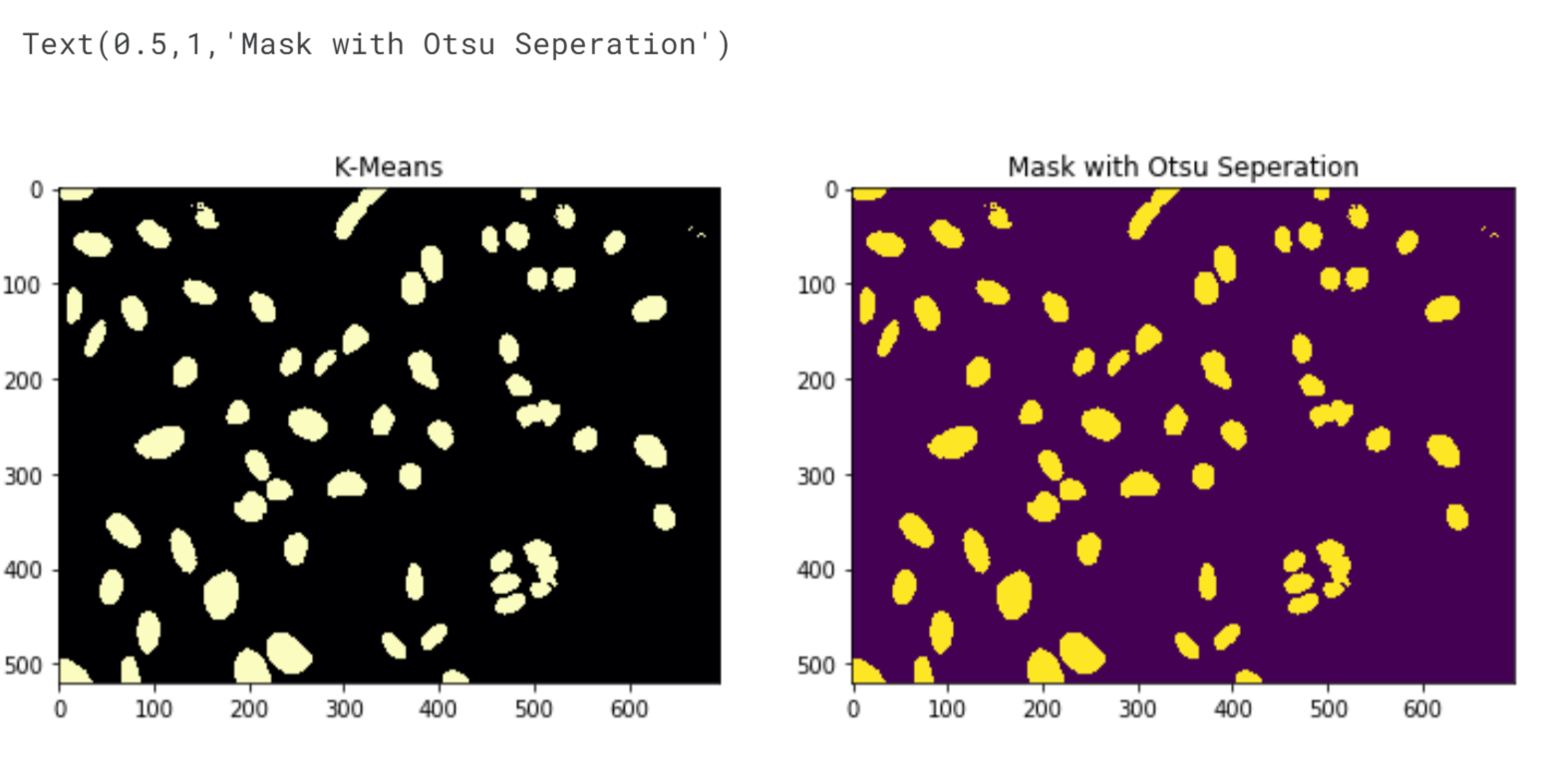e if K-Means does a good job on this data 
from sklearn.cluster import KMeans
kmeans=KMeans(n_clusters=2) #2 as we're still trying to separate the lighter coloured nuclei from the darker coloured background 
kmeans.fit(grayimg.reshape(grayimg.shape[0]*grayimg.shape[1],1))

plt.figure(figsize=(12,6))
plt.subplot(1,2,1)
plt.imshow(kmeans.labels_.reshape(520,696),cmap='magma')
plt.title('K-Means')

plt.subplot(1,2,2)
plt.imshow(maskimg, cmap='viridis')
plt.title('Mask with Otsu Seperation')

Output:

To determine if there is any difference between the labels obtained from Otsu's method and K-Means clustering at a pixel level, we can compare the labels and calculate the percentage of matching labels. If the resulting percentage is 1, it means there is no difference at all.

#To check if there's any difference
sum((kmeans.labels_.reshape(520,696)==mask).flatten())/(mask.shape[0]*mask.shape[1])

Output:

There is no difference at all.

Object Identification

To get a count of the total number of nuclei, we can use the ndimage.label function, which labels features (pixels) in an array based on their interconnectedness. So, for example, if [1 1 1 0 0 1 1] was our row vector, using ndimage.label on this would give us [1 1 1 0 0 2 2] signifying the fact that there are 2 distinct objects in the row vector. The function returns the labelled array and the number of distinct objects it found in the array.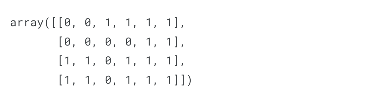

from scipy import ndimage
#To see this at a matrix level
matrix = np.array([[0,0,1,1,1,1],
                  [0,0,0,0,1,1],
                  [1,1,0,1,1,1],
                  [1,1,0,1,1,1]])
matrix

Output:

#Applying the ndimage.label function
ndimage.label(matrix)

Output:

labels,nlabels=ndimage.label(mask)
print('There are',nlabels,'distinct nuclei in the mask.')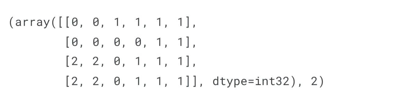

Output:

It is possible that there are more nuclei present in the image than we have currently identified. Some nuclei have merged together, causing them to be counted as a single object in our mask. Additionally, our mask may not have successfully detected all the nuclei, particularly those located in the top right corner. Interestingly, in the top right corner, there are two separate spots that have been labelled as distinct objects, even though they are part of the same group or cluster.

Some insignificant spots or dots are mistakenly labelled as nuclei. To address this issue, we can assign the labels (both from K-Means and Otsu) of these small spots to 0 if their sizes are below a certain threshold. This problem arises because certain nuclei have pixels with intensity values lower than Otsu's threshold, resulting in only some pixels being labelled as 1. By considering the size of the spots and setting their labels to 0 if they are too small, we can ensure that only significant nuclei are accurately identified and labelled.
When nuclei are located close to each other, they tend to be grouped together as a single nucleus. To address this issue, we can employ an edge detection algorithm such as the Sobel filter or Canny edge detector. These algorithms can help identify the boundaries or edges between objects in an image.

By applying the Sobel filter or Canny edge detector, we can detect the edges separating the clustered nuclei. This allows us to distinguish individual nuclei and separate them based on the detected edges. The resulting segmentation will enable more accurate identification and delineation of each nucleus, even when they are in close proximity to one another.

To obtain separate masks for each nucleus, we can utilize the "stage1_train_labels.csv.zip" file, which contains the image IDs and the Run Length Encoded (RLE) vectors corresponding to each nucleus's mask. The RLE vector represents the locations of the pixels within the mask.

#Since w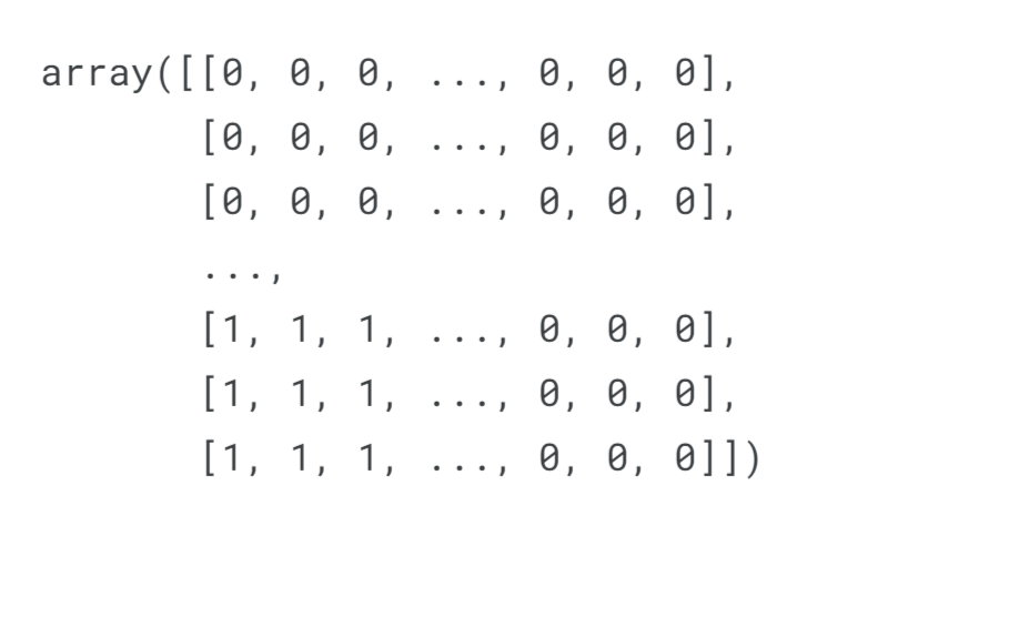e need to create a separate mask for every nucleus, let's store  the masks in an iterable like a list 
label_array=[]
#We need to iterate from 1 as ndimage.label encodes every object starting from number 1
for i in range(1,nlabels+1):
    label_mask = np.where(labels==i,1,0)
    label_array.append(label_mask)
#To see one such mask
label_array[68]

Output:

The 1s represent 1 such object (nucleus) in the entire picture.

Run Length Encoding

RLE or Run Length Encoding converts a matrix into a vector and returns the position/starting point of the first pixel from where we observe an object (identified by a 1) and gives us a count of how many pixels from that pixel we see the series of 1s. In the ndimage.label function example of [1 1 1 0 0 1 1], running RLE would give us 1 3 6 2, which means 3 pixels from the zeroth pixel (inclusive) and 2 pixels from the 5th pixel we see a series of 1s.

#Functi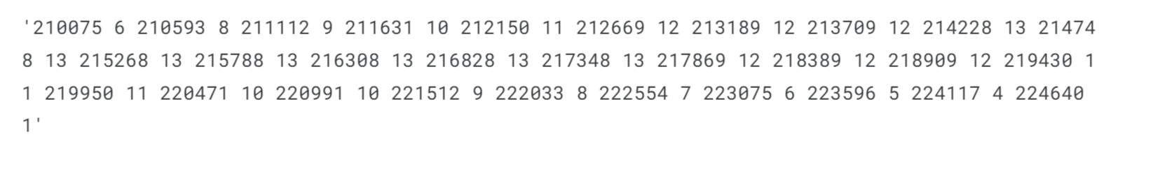on for rle encoding
def rle(x):
    '''
    x: numpy array of shape (height, width), 1 - mask, 0 - background
    Returns run length as list
    '''
    dots = np.where(x.T.flatten()==1)[0] # .T sets Fortran order down-then-right
    run_lengths = []
    prev = -2
    for b in dots:
        if (b>prev+1): run_lengths.extend((b+1, 0))
        run_lengths[-1] += 1
        prev = b
    return " ".join([str(i) for i in run_lengths])

#Running RLE on the last label_mask in label_array gives us 
rle(label_mask)

Output:

Merging Everything Together

#To take a look at the different parts
im_path.parts

Output:

#Now defining a function that is applicable to all images
def basic(im_path):
    #Reading the image
    im_id=im_path.parts[-3] #To extract the image ID
    bgr = cv2.imread(str(im_path)) #Reading it in OpenCV
    gray = cv2.cvtColor(bgr,cv2.COLOR_BGR2GRAY) #Converting everything to grayscale from BGR

    #To remove the background
    thresh_val = threshold_otsu(gray) #Using Otsu's method to separate the foreground objects from the background
    mask = np.where(gray > thresh_val, 1, 0) #Coding objects with intensity values higher than background as 1
    
    #Extracting connected objects
    test_rle=pd.DataFrame()
    labels, nlabels = ndimage.label(mask) #labels give us the label of the different objects in every image starting from 1 ,and nlabels gives us the total number of objects in every image
    for i in range(1,nlabels+1): #Iterating through every object/label
        label_mask = np.where(labels==i,1,0) #Individual masks for every nucleus
        RLE = rle(label_mask) #RLE for every mask
        solution = pd.Series({'ImageId': im_id, 'EncodedPixels': RLE})
        test_rle = test_rle.append(solution, ignore_index=True)
    
    #Return the dataframe
    return(test_rle)

#Defining a function that takes a list of image paths (pathlib.Path objects), analyzes each and returns a submission ready DataFrame
def list_of_images(im_path_list):
    all_df = pd.DataFrame()
    for im_path in im_path_list: #We'll use this for the test images
        im_df = basic(im_path) #Creating one dataframe for every image 
        all_df = all_df.append(im_df, ignore_index=True) #Appending all these dataframes
    
    #Returing the submission ready dataframe
    return (all_df)

Edge Detection

Edge detection is a fundamental concept in image processing that involves identifying boundaries or edges between different objects or regions within an image. It plays a vital role in various fields, such as computer vision, robotics, and medical imaging. Traditional edge detection algorithms, like the Sobel operator and the Canny edge detector, use mathematical operations to locate areas of rapid-intensity transitions.

Here, we will use the Sobel Filter first.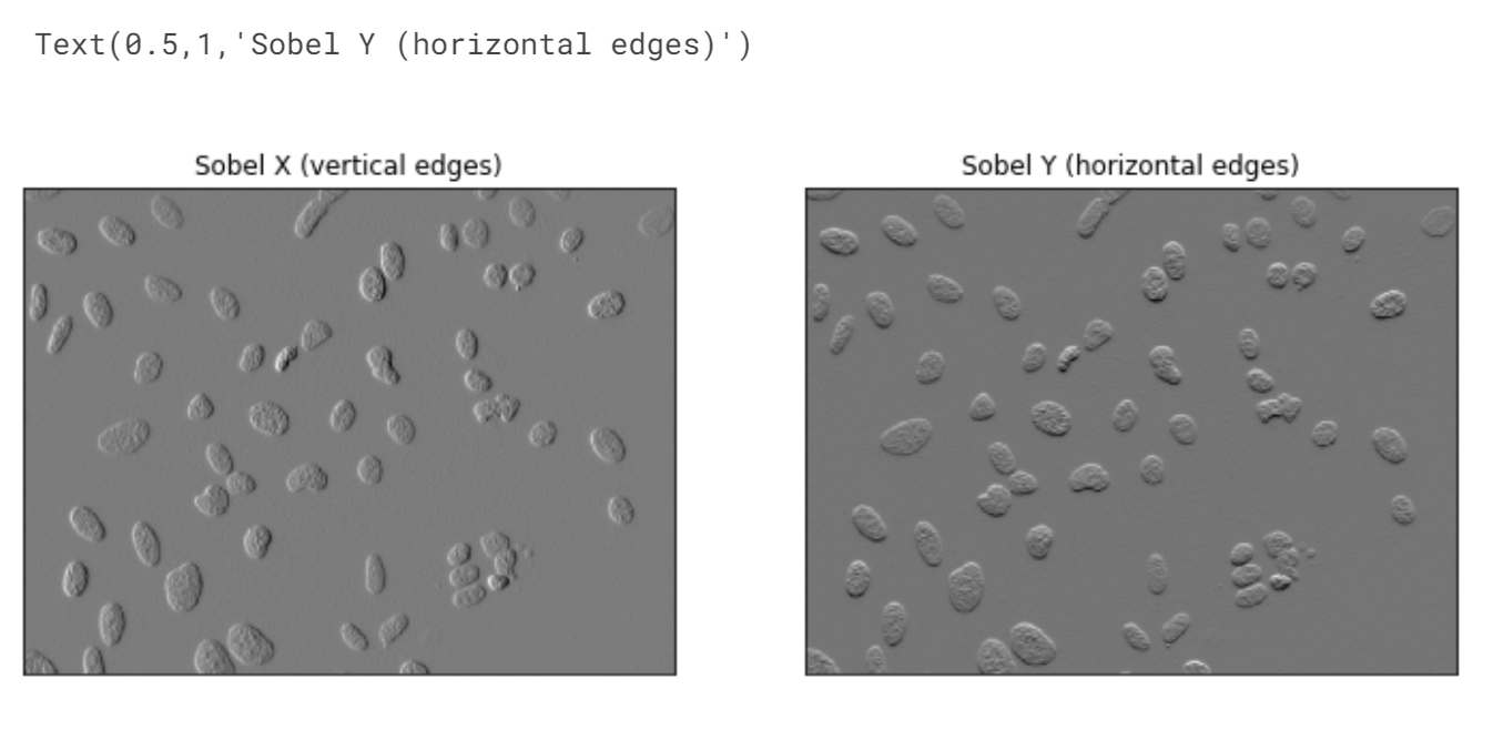

#cv2.Sobel arguments - the image, output depth, order of derivative of x, order of derivative of y, kernel/filter matrix size
sobelx = cv2.Sobel(grayimg,int(cv2.CV_64F),1,0,ksize=3) #ksize=3 means we'll be using the 3x3 Sobel filter
sobely = cv2.Sobel(grayimg,int(cv2.CV_64F),0,1,ksize=3)

#To plot the vertical and horizontal edge detectors side by side
plt.figure(figsize=(12,6))
plt.subplot(1,2,1)
plt.imshow(sobelx,cmap='gray')
plt.title('Sobel X (vertical edges)')
plt.xticks([])
plt.yticks([])

plt.subplot(1,2,2)
plt.imshow(sobely,cmap='gray')
plt.xticks([])
plt.yticks([])
plt.title('Sobel Y (horizontal edges)')

Output:

#Plotting the original image
plt.figure(figsize=(12,6))
plt.subplot(1,2,1)
plt.imshow(grayimg,cmap='gray')
plt.title('Original image')

#Now to combine the 2 sobel filters
sobel = np.sqrt(np.square(sobelx) + np.square(sobely))
plt.subplot(1,2,2)
plt.imshow(sobel,cmap='gray')
plt.title('Sobel Filter')

Output: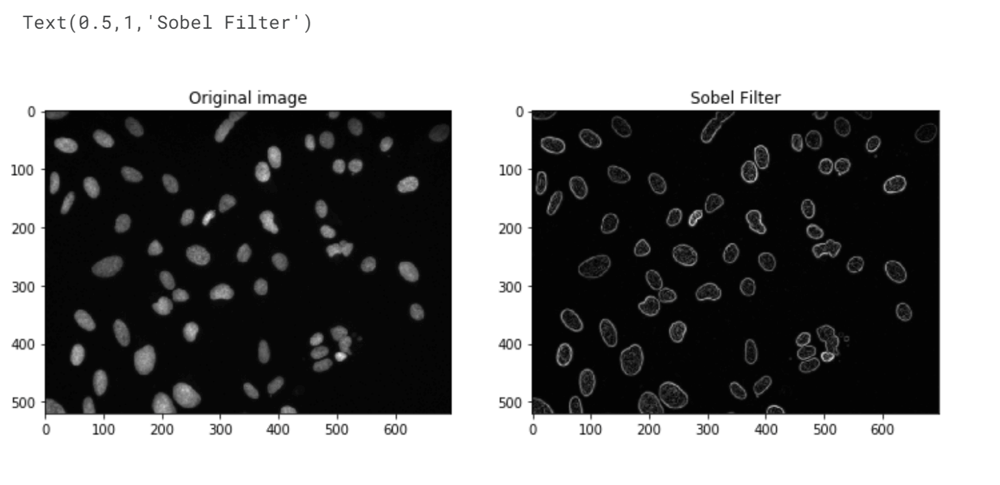

The Sobel filter has performed better than Otsu/K-Means in identifying separate objects in the image. It successfully detected the two nuclei in the top right corner and the two small nuclei near the (530,410) area. However, there is still room for improvement as it merged two out of the three overlapping nuclei in that region instead of recognizing them as separate objects.

#To high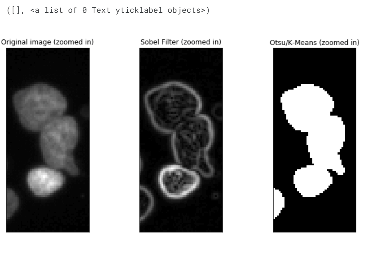light the problem areas
plt.figure(figsize=(12,6))
plt.subplot(1,3,1)
plt.imshow(grayimg[350:450,485:530],cmap='gray')
plt.title('Original image (zoomed in)')
plt.xticks([])
plt.yticks([])

plt.subplot(1,3,2)
plt.imshow(sobel[350:450,485:530],cmap='gray')
plt.title('Sobel Filter (zoomed in)')
plt.xticks([])
plt.yticks([])

plt.subplot(1,3,3)
plt.imshow(maskimg[350:450,485:530], cmap='gray')
plt.title('Otsu/K-Means (zoomed in)')
plt.xticks([])
plt.yticks([])

Output:

We will now employ a Canny edge detector which is a smarter Sobel Filter.

plt.fig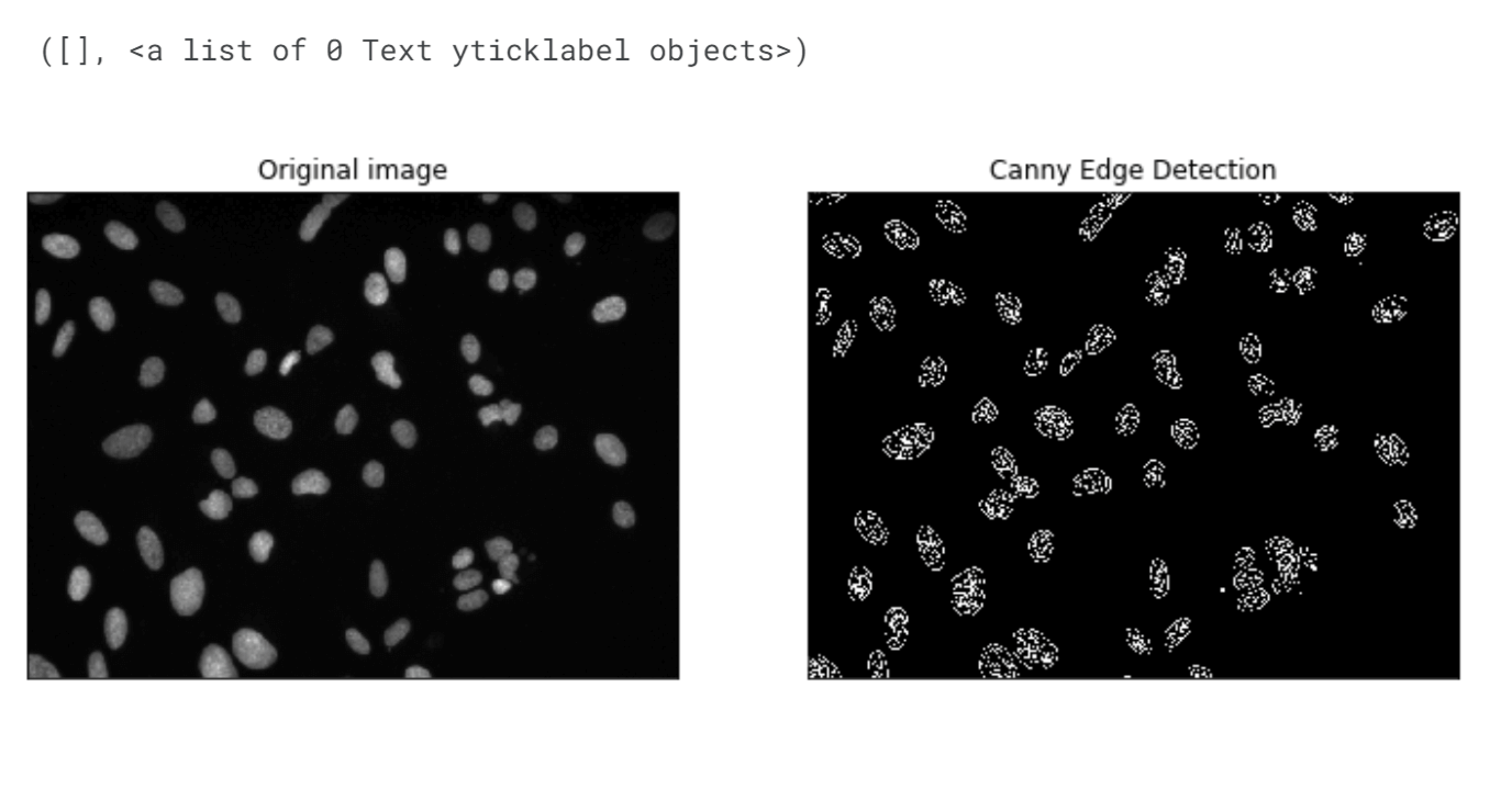ure(figsize=(12,6))

plt.subplot(1,2,1)
plt.imshow(grayimg,cmap='gray')
plt.title('Original image')
plt.xticks([])
plt.yticks([])

#Let's see how the Canny Edge Detector does on the image
plt.subplot(1,2,2)
canny = cv2.Canny(grayimg,0,21)
plt.imshow(canny,cmap='gray')
plt.title('Canny Edge Detection')
plt.xticks([])
plt.yticks([])

Output:

The Canny Edge Detector has detected gradients within the nuclei, which may seem excessive. However, if we focus on extracting only the external contours and use them to create masks, we can capture the regions of interest more accurately. It's important to note that similar issues to those encountered with the Sobel filter persist here. Nevertheless, the Canny Edge Detector generates a modified image matrix consisting of binary values (0 and 255), simplifying the representation of the detected edges.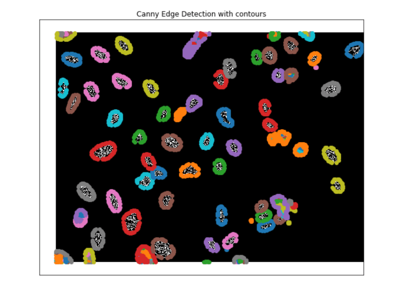

#Using contouring to create the masks
canny_cont=cv2.findContours(canny,cv2.RETR_EXTERNAL,cv2.CHAIN_APPROX_SIMPLE)[1] #Using an approximation function to obtain the contour points and retrieving only the external contours

#To show the contour points
plt.figure(figsize=(14,8))
plt.imshow(canny,cmap='gray')
plt.title('Canny Edge Detection with contours')
plt.xticks([])
plt.yticks([])

for i in (range(len(canny_cont))):
    plt.scatter(canny_cont[i].flatten().reshape(len(canny_cont[i]),2)[:,0],
         canny_cont[i].flatten().reshape(len(canny_cont[i]),2)[:,1])

Output:

plt.figure(figsize=(12,6))
plt.subplot(1,2,1)
plt.imshow(grayimg, cmap='gray')
plt.title('Original Image')

#Now to create masks with contours
background=np.zeros(grayimg.shape)
canny_mask=cv2.drawContours(background,canny_cont,-1,255,-1)

plt.subplot(1,2,2)
plt.imshow(canny_mask,cmap='gray')
plt.title('Creating masks with contours')
plt.xticks([])
plt.yticks([])

Output: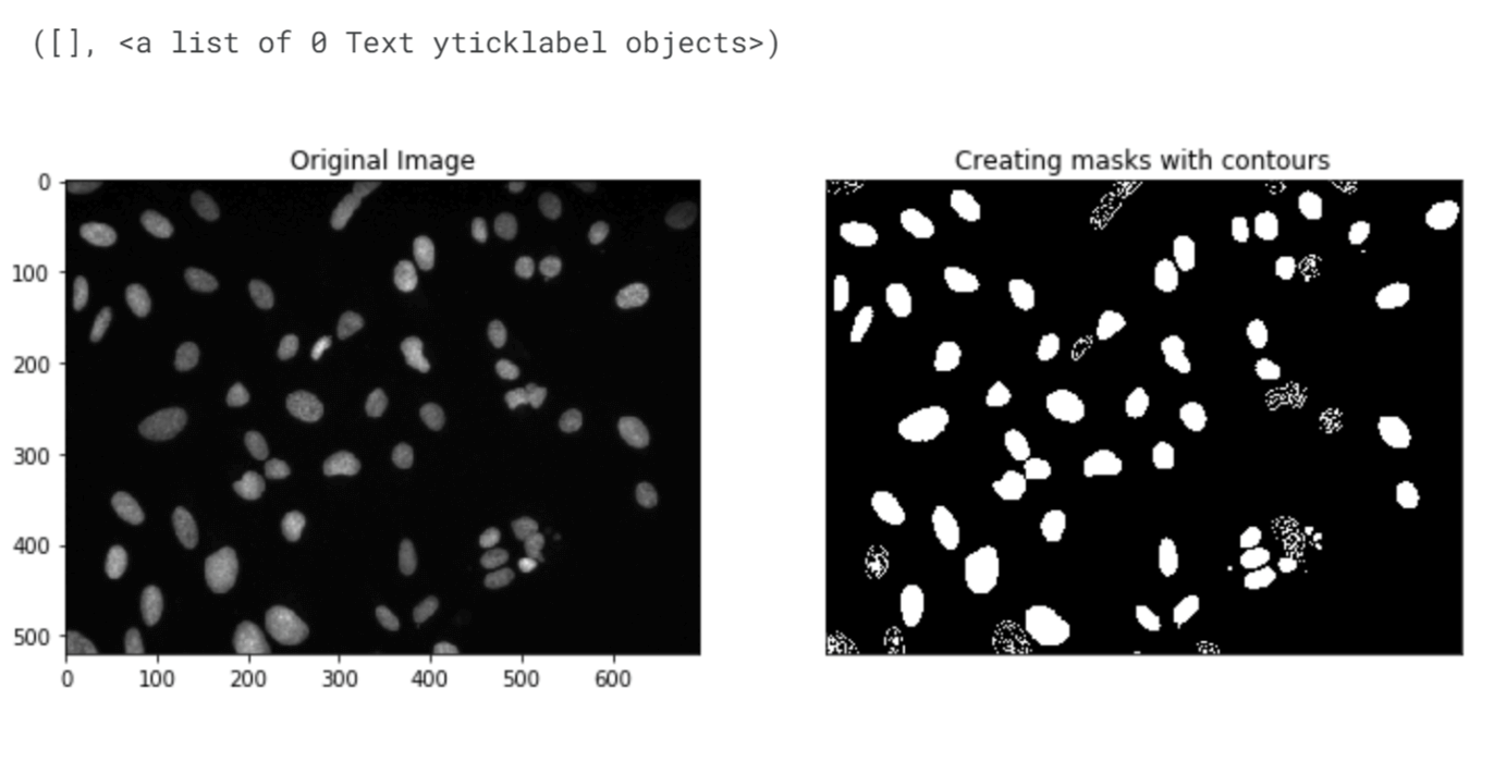

The Canny Edge Detector has successfully detected most of the nuclei, but complete masks for each nucleus are not obtained. Adjusting the minval and maxval parameters in the cv2.Canny() function can potentially improve the results, taking into account the specific characteristics of the image being processed. The canny_mask matrix output is compatible with the ndimage.labels function, which is used to identify connected components. However, it is crucial to generate complete masks for each nucleus to ensure that we do not detect more objects than are actually present in the image.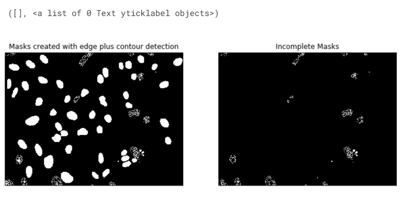

canny_mask_copy=canny_mask.copy()
canny_mask_clabels=ndimage.label(canny_mask_copy)[0]
for label_ind, label_mat in enumerate(ndimage.find_objects(canny_mask_clabels)):
    cell = canny_mask_clabels[label_mat]
    #Toheck if the label size is too small
    if np.product(cell.shape) < 100:
        canny_mask_clabels[np.where(canny_mask_clabels==label_ind+1)]=1
canny_mask_clabels=np.where(canny_mask_clabels>1,0,canny_mask_clabels)

#To show the original mask
plt.figure(figsize=(12,6))
plt.subplot(1,2,1)
plt.imshow(canny_mask,cmap='gray')
plt.title('Masks created with edge plus contour detection')
plt.xticks([])
plt.yticks([])

#To plot the problem areas
plt.subplot(1,2,2)
plt.imshow(canny_mask_clabels,cmap='gray')
plt.title('Incomplete Masks')
plt.xticks([])
plt.yticks([])

Output:

#For convolving 2D arrays
from scipy import signal
plt.figure(figsize=(12,6))
plt.subplot(1,2,1)
sns.distplot(np.where(canny_mask==255,1,0).flatten())
plt.title('Canny Mask')

plt.subplot(1,2,2)
#To smooth the canny_mask by convolving with a matrix that has all values = 1/9
canny_mask_smooth=signal.convolve2d(np.where(canny_mask==255,1,0),np.full((3,3),1/9),'same')
sns.distplot(canny_mask_smooth.flatten())
canny_mask_smooth_thresh=threshold_otsu(canny_mask_smooth)
plt.axvline(x=canny_mask_smooth_thresh)
plt.title('Smoothened Canny Mask with Otsu threshold value')

Output: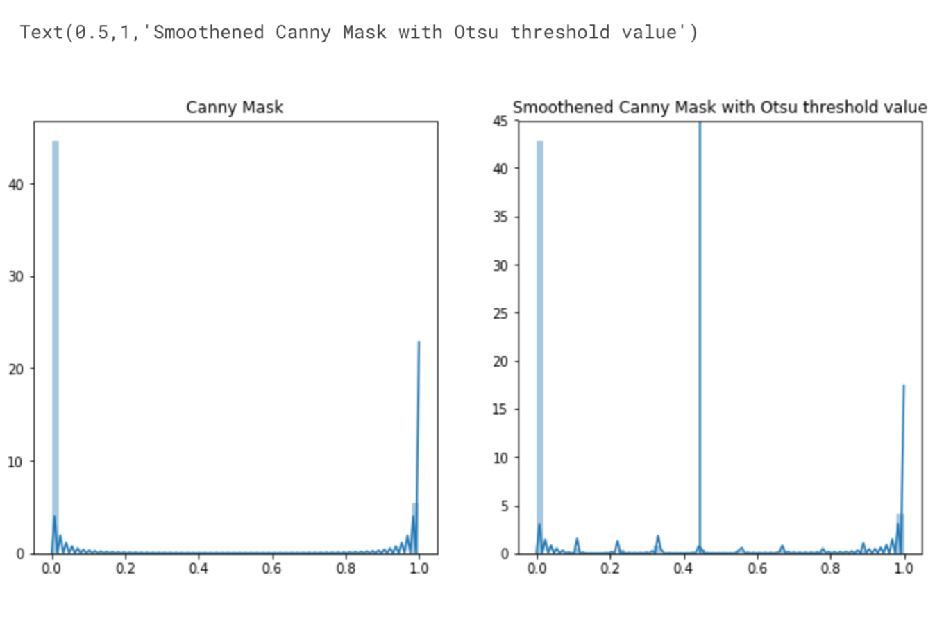

The number of pixels with intensity values equal to 1 has decreased. This reduction is attributed to the smoothing process. We performed convolution on the canny mask using a local filter, specifically a 3x3 matrix where all values are set to 1/9. This operation replaces the intensity values of the pixels with the average intensity value of their neighbouring pixels. If a pixel is surrounded by neighbouring pixels with intensity values of 1, its intensity value remains as 1 (since 1/9 multiplied by 9 equals 1). However, the pixels located at the edges of objects and in problematic areas experience a decrease in their intensity values.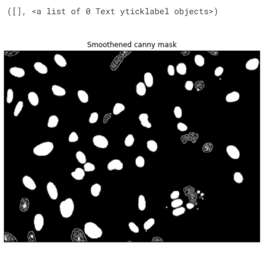

plt.figure(figsize=(12,6))
plt.imshow(canny_mask_smooth,cmap='gray')
plt.title('Smoothened canny mask')
plt.xticks([])
plt.yticks([])

Output:

#Setting all values above otsu's threshold as 0 in the matrix and in this image matrix setting all values above 0 as 1 
plt.figure(figsize=(12,6))
canny_conv1=np.where(np.where(canny_mask_smooth>canny_mask_smooth_thresh,0,canny_mask_smooth)>0,1,0)
plt.imshow(canny_conv1,cmap='gray')
plt.xticks([])
plt.yticks([])
plt.title('After 1 convolution')

Output:

plt.figure(figsize=(12,6))
canny_mask_smooth2=signal.convolve2d(canny_conv1,np.full((3,3),1/9),'same')
canny_mask_smooth_thresh2=threshold_otsu(canny_mask_smooth2)
canny_conv2=np.where(canny_mask_smooth2>canny_mask_smooth_thresh2,1,0)
plt.imshow(canny_conv2,cmap='gray')
plt.xticks([])
plt.yticks([])
plt.title('After 2 convolutions')

Output:

#Combing the 2 convolutions 
canny_cont=cv2.findContours(cv2.convertScaleAbs(canny_conv2),cv2.RETR_EXTERNAL,cv2.CHAIN_APPROX_SIMPLE)[1]
background=np.zeros(grayimg.shape)
canny_mask=cv2.drawContours(background,canny_cont,-1,255,-1)

plt.figure(figsize=(12,6))
plt.imshow(canny_mask,cmap='gray')
plt.title('Contour detection after 2 convolutions')
plt.xticks([])
plt.yticks([])

Output: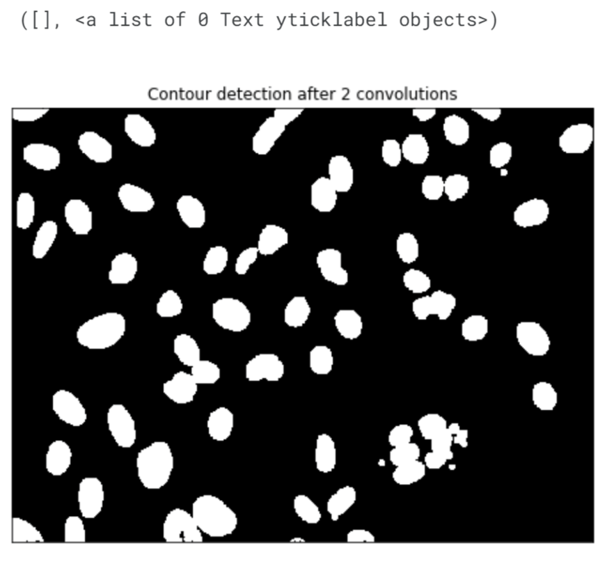

Overall, the current results are satisfactory. Although there are still instances where nuclei are clustered together, the important point is that we have successfully identified all the nuclei in the original image. However, before proceeding further and potentially overfitting to a specific image, it is crucial to explore different values for the MinVal and MaxVal parameters in the cv2.Canny() function to determine their effectiveness on other images. This allows us to establish a more robust approach that can generalize well across various scenarios.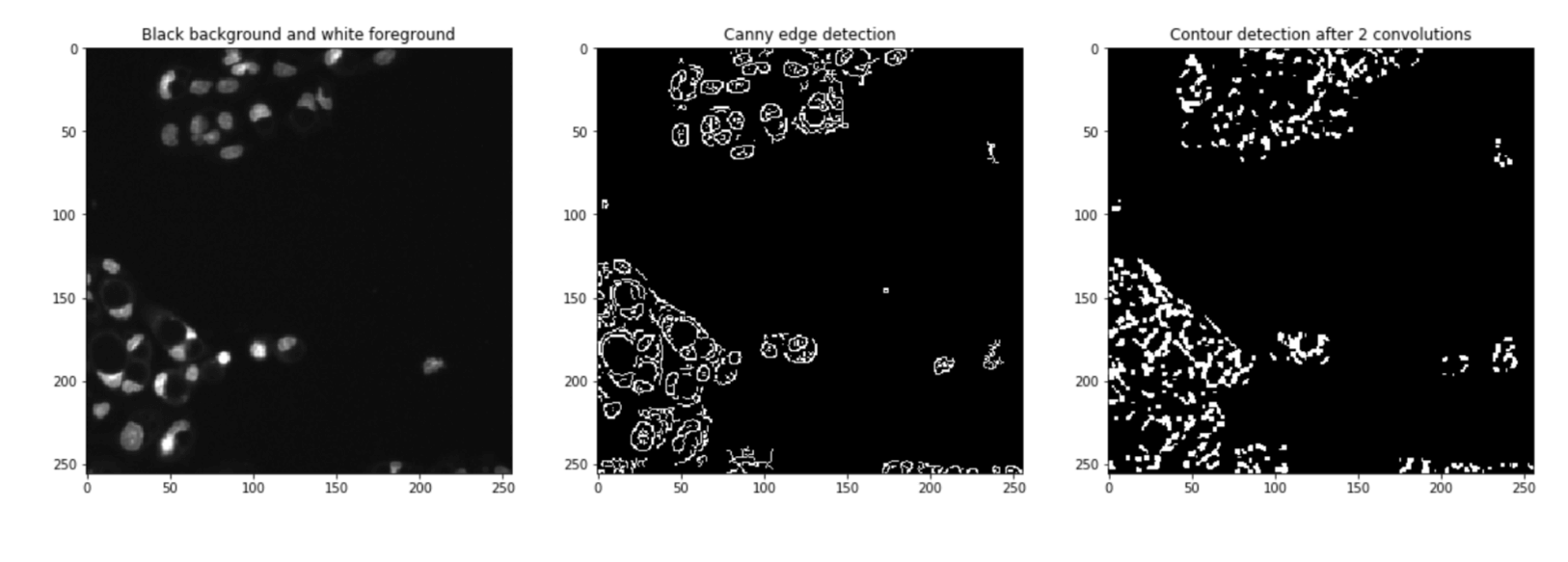

#Let's try the same parameters for the canny edge on other types of images - starting with another black background and white foreground image
for i in range(len(training_sorted)):
    if training_sorted[i].parts[-1]=='feffce59a1a3eb0a6a05992bb7423c39c7d52865846da36d89e2a72c379e5398.png':
        bwimg=cv2.imread(str(training_sorted[i]))
        bwimg=cv2.cvtColor(bwimg,cv2.COLOR_BGR2RGB)
        plt.figure(figsize=(20,8))
        plt.subplot(1,3,1)
        plt.imshow(bwimg)
        plt.title('Black background and white foreground')
        
        plt.subplot(1,3,2)
        bwimg=cv2.cvtColor(bwimg,cv2.COLOR_RGB2GRAY)
        bwimg_canny=cv2.Canny(bwimg,0,21)
        plt.imshow(bwimg_canny,cmap='gray')
        plt.title('Canny edge detection')
        
        plt.subplot(1,3,3)
        bwimg_cont=cv2.findContours(bwimg_canny,cv2.RETR_EXTERNAL,cv2.CHAIN_APPROX_SIMPLE)[1]
        #Now to create masks with contours
        bwimg_bg=np.zeros(bwimg.shape)
        bwimg_mask=cv2.drawContours(bwimg_bg,bwimg_cont,-1,255,-1)
        
        #Convolving once
        bwimg_mask_smooth=signal.convolve2d(np.where(bwimg_mask==255,1,0),np.full((3,3),1/9),'same')
        bwimg_mask_smooth_thresh=threshold_otsu(bwimg_mask_smooth)
        bwimg_conv1=np.where(np.where(bwimg_mask_smooth>bwimg_mask_smooth_thresh,0,bwimg_mask_smooth)>0,1,0)
        
        #Convolving again
        bwimg_mask_smooth2=signal.convolve2d(bwimg_conv1,np.full((3,3),1/9),'same')
        bwimg_mask_smooth_thresh2=threshold_otsu(bwimg_mask_smooth2)
        bwimg_conv2=np.where(bwimg_mask_smooth2>bwimg_mask_smooth_thresh2,1,0)
        
        #Now to create masks with contours after 2 convolutions
        bwimg_cont=cv2.findContours(cv2.convertScaleAbs(bwimg_conv2),cv2.RETR_EXTERNAL,cv2.CHAIN_APPROX_SIMPLE)[1]
        bwimg_bg=np.zeros(bwimg.shape)
        bwimg_mask=cv2.drawContours(bwimg_bg,bwimg_cont,-1,255,-1)

        plt.imshow(bwimg_mask,cmap='gray')
        plt.title('Contour detection after 2 convolutions')

Output:

#Purple background and purple foreground
for i in range(len(training_sorted)):
    if training_sorted[i].parts[-1]=='0e21d7b3eea8cdbbed60d51d72f4f8c1974c5d76a8a3893a7d5835c85284132e.png':
        ppimg=cv2.imread(str(training_sorted[i]))
        ppimg=cv2.cvtColor(ppimg,cv2.COLOR_BGR2RGB)
        plt.figure(figsize=(20,8))
        plt.subplot(1,3,1)
        plt.imshow(ppimg)
        plt.title('Purple background and purple foreground')
        
        plt.subplot(1,3,2)
        ppimg=cv2.cvtColor(ppimg,cv2.COLOR_RGB2GRAY)
        ppimg_canny=cv2.Canny(ppimg,20,100)
        plt.imshow(ppimg_canny,cmap='gray')
        plt.title('Canny edge detection')
        
        plt.subplot(1,3,3)
        ppimg_cont=cv2.findContours(ppimg_canny,cv2.RETR_EXTERNAL,cv2.CHAIN_APPROX_SIMPLE)[1]
        #Now to create masks with contours
        ppimg_bg=np.zeros(ppimg.shape)
        ppimg_mask=cv2.drawContours(ppimg_bg,ppimg_cont,-1,255,-1)
        
        #Convolving once
        ppimg_mask_smooth=signal.convolve2d(np.where(ppimg_mask==255,1,0),np.full((3,3),1/9),'same')
        ppimg_mask_smooth_thresh=threshold_otsu(ppimg_mask_smooth)
        ppimg_conv1=np.where(np.where(ppimg_mask_smooth>ppimg_mask_smooth_thresh,0,ppimg_mask_smooth)>0,1,0)
        
        #Convolving again
        ppimg_mask_smooth2=signal.convolve2d(ppimg_conv1,np.full((3,3),1/9),'same')
        ppimg_mask_smooth_thresh2=threshold_otsu(ppimg_mask_smooth2)
        ppimg_conv2=np.where(ppimg_mask_smooth2>ppimg_mask_smooth_thresh2,1,0)
        
        #Now to create masks with contours after 2 convolutions
        ppimg_cont=cv2.findContours(cv2.convertScaleAbs(ppimg_conv2),cv2.RETR_EXTERNAL,cv2.CHAIN_APPROX_SIMPLE)[1]
        ppimg_bg=np.zeros(ppimg.shape)
        ppimg_mask=cv2.drawContours(ppimg_bg,ppimg_cont,-1,255,-1)

        plt.imshow(ppimg_mask,cmap='gray')
        plt.title('Contour detection after 2 convolutions')

Output:

#White background and purple foreground
for i in range(len(training_sorted)):
    if training_sorted[i].parts[-1]=='0121d6759c5adb290c8e828fc882f37dfaf3663ec885c663859948c154a443ed.png':
        wpimg=cv2.imread(str(training_sorted[i]))
        wpimg=cv2.cvtColor(wpimg,cv2.COLOR_BGR2RGB)
        plt.figure(figsize=(20,8))
        plt.subplot(1,3,1)
        plt.imshow(wpimg)
        plt.title('White background and purple foreground')
        
        plt.subplot(1,3,2)
        wpimg=cv2.cvtColor(wpimg,cv2.COLOR_RGB2GRAY)
        wpimg_canny=cv2.Canny(wpimg,20,100)
        plt.imshow(wpimg_canny,cmap='gray')
        plt.title('Canny edge detection')
        
        plt.subplot(1,3,3)
        wpimg_cont=cv2.findContours(wpimg_canny,cv2.RETR_EXTERNAL,cv2.CHAIN_APPROX_SIMPLE)[1]
        #Now to create masks with contours
        wpimg_bg=np.zeros(wpimg.shape)
        wpimg_mask=cv2.drawContours(wpimg_bg,wpimg_cont,-1,255,-1)
        
        #Convolving once
        wpimg_mask_smooth=signal.convolve2d(np.where(wpimg_mask==255,1,0),np.full((3,3),1/9),'same')
        wpimg_mask_smooth_thresh=threshold_otsu(wpimg_mask_smooth)
        wpimg_conv1=np.where(np.where(wpimg_mask_smooth>wpimg_mask_smooth_thresh,0,wpimg_mask_smooth)>0,1,0)
        
        #Convolving again
        wpimg_mask_smooth2=signal.convolve2d(wpimg_conv1,np.full((3,3),1/9),'same')
        wpimg_mask_smooth_thresh2=threshold_otsu(wpimg_mask_smooth2)
        wpimg_conv2=np.where(wpimg_mask_smooth2>wpimg_mask_smooth_thresh2,1,0)
        
        #Now to create masks with contours after 2 convolutions
        wpimg_cont=cv2.findContours(cv2.convertScaleAbs(wpimg_conv2),cv2.RETR_EXTERNAL,cv2.CHAIN_APPROX_SIMPLE)[1]
        wpimg_bg=np.zeros(wpimg.shape)
        wpimg_mask=cv2.drawContours(wpimg_bg,wpimg_cont,-1,255,-1)

        plt.imshow(wpimg_mask,cmap='gray')
        plt.title('Contour detection after 2 convolutions')

Output:

#White background and black foreground
for i in range(len(training_sorted)):
    if training_sorted[i].parts[-1]=='08275a5b1c2dfcd739e8c4888a5ee2d29f83eccfa75185404ced1dc0866ea992.png':
        wbimg=cv2.imread(str(training_sorted[i]))
        wbimg=cv2.cvtColor(wbimg,cv2.COLOR_BGR2RGB)
        plt.figure(figsize=(20,8))
        plt.subplot(1,3,1)
        plt.imshow(wbimg)
        plt.title('White background and black foreground')
        
        plt.subplot(1,3,2)
        wbimg=cv2.cvtColor(wbimg,cv2.COLOR_RGB2GRAY)
        wbimg_canny=cv2.Canny(wbimg,20,100)
        plt.imshow(wbimg_canny,cmap='gray')
        plt.title('Canny edge detection')
        
        plt.subplot(1,3,3)
        wbimg_cont=cv2.findContours(wbimg_canny,cv2.RETR_EXTERNAL,cv2.CHAIN_APPROX_SIMPLE)[1]
        #Now to create masks with contours
        wbimg_bg=np.zeros(wbimg.shape)
        wbimg_mask=cv2.drawContours(wbimg_bg,wbimg_cont,-1,255,-1)
        
        #Convolving once
        wbimg_mask_smooth=signal.convolve2d(np.where(wbimg_mask==255,1,0),np.full((5,5),1/25),'same')
        wbimg_mask_smooth_thresh=threshold_otsu(wbimg_mask_smooth)
        wbimg_conv1=np.where(np.where(wbimg_mask_smooth>wbimg_mask_smooth_thresh,0,wbimg_mask_smooth)>0,1,0)
        
        #Convolving again
        wbimg_mask_smooth2=signal.convolve2d(wbimg_conv1,np.full((5,5),1/25),'same')
        wbimg_mask_smooth_thresh2=threshold_otsu(wbimg_mask_smooth2)
        wbimg_conv2=np.where(wbimg_mask_smooth2>wbimg_mask_smooth_thresh2,1,0)
        
        #Now to create masks with contours after 2 convolutions
        wbimg_cont=cv2.findContours(cv2.convertScaleAbs(wbimg_conv2),cv2.RETR_EXTERNAL,cv2.CHAIN_APPROX_SIMPLE)[1]
        wbimg_bg=np.zeros(wbimg.shape)
        wbimg_mask=cv2.drawContours(wbimg_bg,wbimg_cont,-1,255,-1)

        plt.imshow(wbimg_conv2,cmap='gray')
        plt.title('Contour detection after 2 convolutions')

Output:

#There are some images in the test set with a yellow background and purple foreground
test_images = pathlib.Path('../input/stage1_test/').glob('*/images/*.png')
testing_sorted=sorted([x for x in test_images])
for i in range(len(testing_sorted)):
    if testing_sorted[i].parts[-1]=='9f17aea854db13015d19b34cb2022cfdeda44133323fcd6bb3545f7b9404d8ab.png':
        ypimg=cv2.imread(str(testing_sorted[i]))
        ypimg=cv2.cvtColor(ypimg,cv2.COLOR_BGR2RGB)
        plt.figure(figsize=(20,8))
        plt.subplot(1,3,1)
        plt.imshow(ypimg)
        plt.title('Yellow background and purple foreground')
        
        plt.subplot(1,3,2)
        ypimg=cv2.cvtColor(ypimg,cv2.COLOR_RGB2GRAY)
        ypimg_canny=cv2.Canny(ypimg,100,200)
        plt.imshow(ypimg_canny,cmap='gray')
        plt.title('Canny edge detection')
        
        plt.subplot(1,3,3)
        ypimg_cont=cv2.findContours(ypimg_canny,cv2.RETR_EXTERNAL,cv2.CHAIN_APPROX_SIMPLE)[1]
        #Now to create masks with contours
        ypimg_bg=np.zeros(ypimg.shape)
        ypimg_mask=cv2.drawContours(ypimg_bg,ypimg_cont,-1,255,-1)
        
        #Convolving once
        ypimg_mask_smooth=signal.convolve2d(np.where(ypimg_mask==255,1,0),np.full((3,3),1/9),'same')
        ypimg_mask_smooth_thresh=threshold_otsu(ypimg_mask_smooth)
        ypimg_conv1=np.where(np.where(ypimg_mask_smooth>ypimg_mask_smooth_thresh,0,ypimg_mask_smooth)>0,1,0)
        
        #Convolving again
        ypimg_mask_smooth2=signal.convolve2d(ypimg_conv1,np.full((3,3),1/9),'same')
        ypimg_mask_smooth_thresh2=threshold_otsu(ypimg_mask_smooth2)
        ypimg_conv2=np.where(ypimg_mask_smooth2>ypimg_mask_smooth_thresh2,1,0)
        
        #Now to create masks with contours after 2 convolutions
        ypimg_cont=cv2.findContours(cv2.convertScaleAbs(ypimg_conv2),cv2.RETR_EXTERNAL,cv2.CHAIN_APPROX_SIMPLE)[1]
        ypimg_bg=np.zeros(ypimg.shape)
        ypimg_mask=cv2.drawContours(ypimg_bg,ypimg_cont,-1,255,-1)

        plt.imshow(ypimg_conv2,cmap='gray')
        plt.title('Contour detection after 2 convolutions')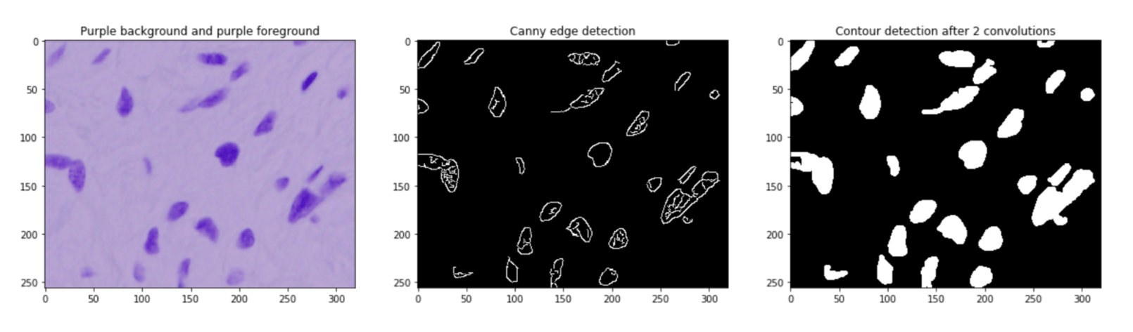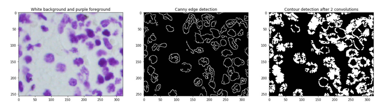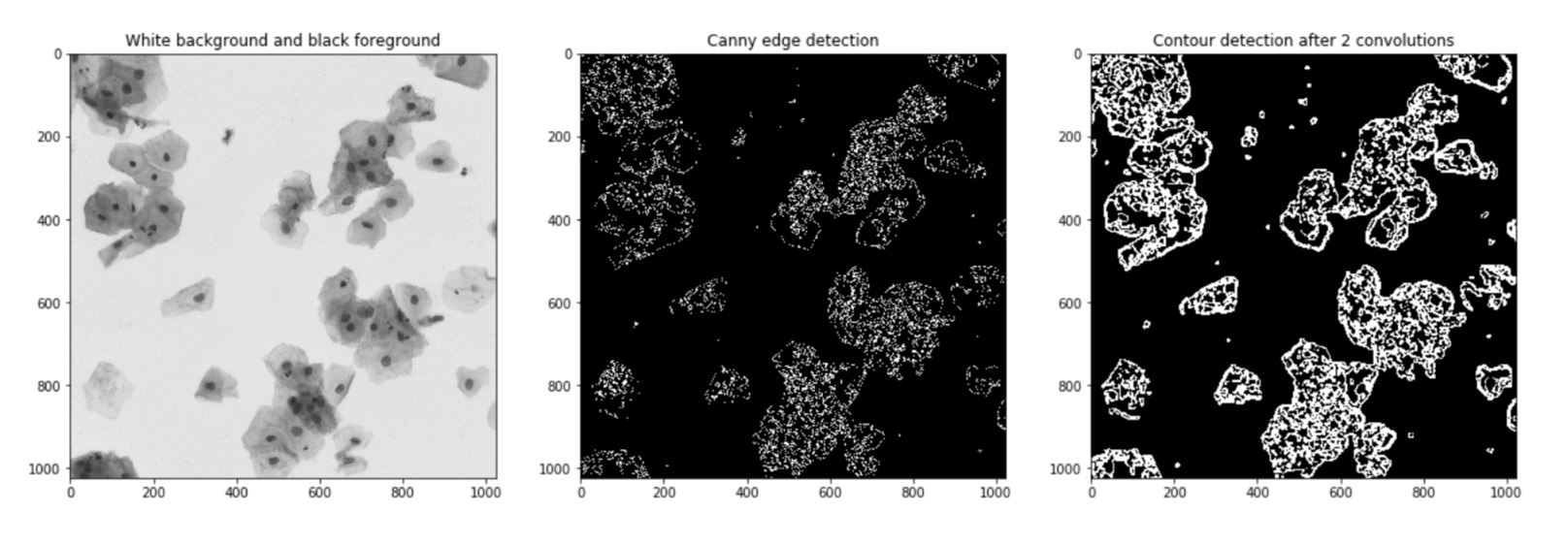

Output: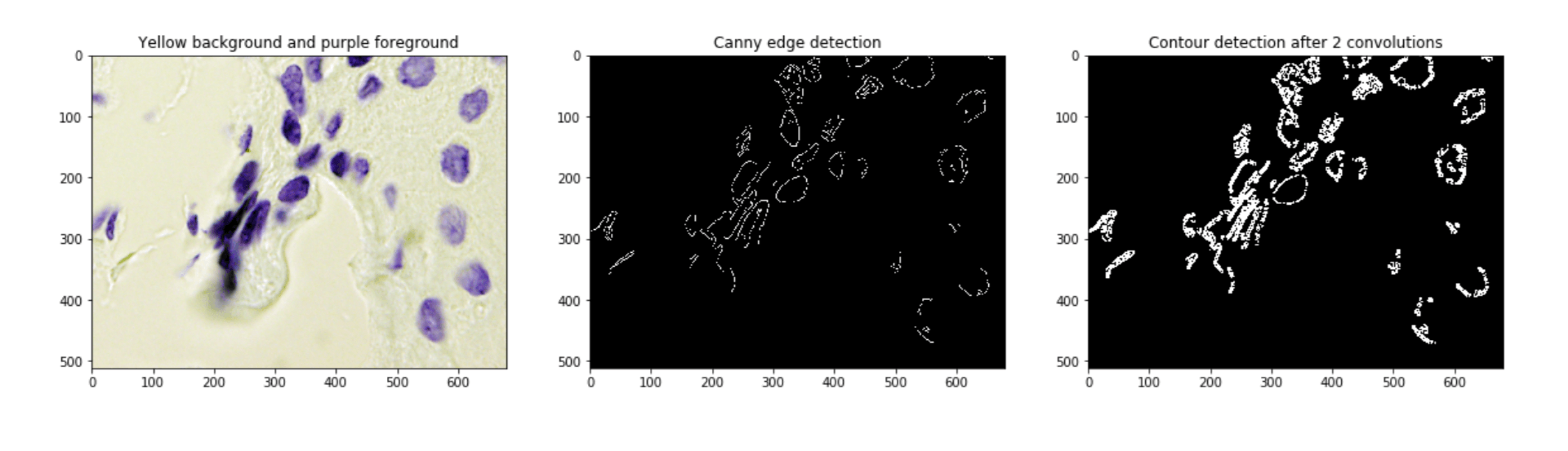

It is not hard to see that the same parameters as on the black background and white foreground images will fail miserably on other kinds of images.

Pixel Classifier

We'll try to build a pixel classifier that classifies pixels as 0 or 255 depending on the grayscale values of the pixel and its neighbours.

train_p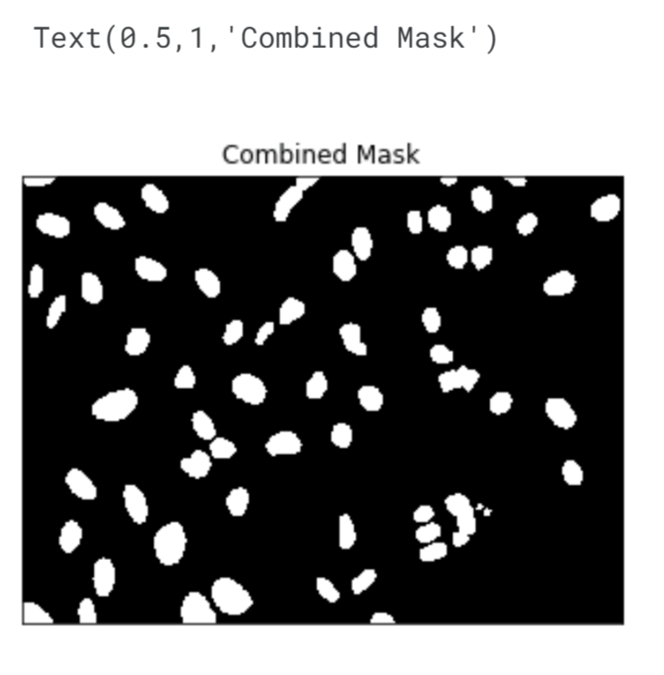ath = '../input/stage1_train/'
test_path = '../input/stage1_test/'
train_ids = os.listdir(train_path)
def LabelMerge(imgpath):
    #to get all the png files
    png_files = [f for f in os.listdir(imgpath) if f.endswith('.png')]
    #to load the image as a grayscale
    img = cv2.imread(imgpath+'/'+png_files[0],0)
    for i in png_files[1:]:
        temp_img = cv2.imread(imgpath+'/'+i,0)
        img = img+temp_img
    return(img)

path = train_path+training_sorted[45].parts[-3]+'/masks/'
combined_mask=LabelMerge(path)
plt.imshow(combined_mask,cmap='gray')
plt.xticks([])
plt.yticks([])
plt.title('Combined Mask')

Output:

We will use the bounding boxes of nuclei found in the mask to localize and classify nuclei in the original image. By considering grayscale values and corresponding labels in the combined mask, we assign labels to pixels within the bounding boxes. While some nuclei may be clustered together or result in false positives, our focus is on regions of interest. The pixel classifier relies on grayscale values and neighbouring pixel information to make accurate classifications. The goal is to ensure that all regions with nuclei are captured, avoiding false negatives while allowing the classifier to assign 0 values to non-nucleus regions. The performance of the pixel classifier depends on the defined features and their ability to accurately classify the pixels.

o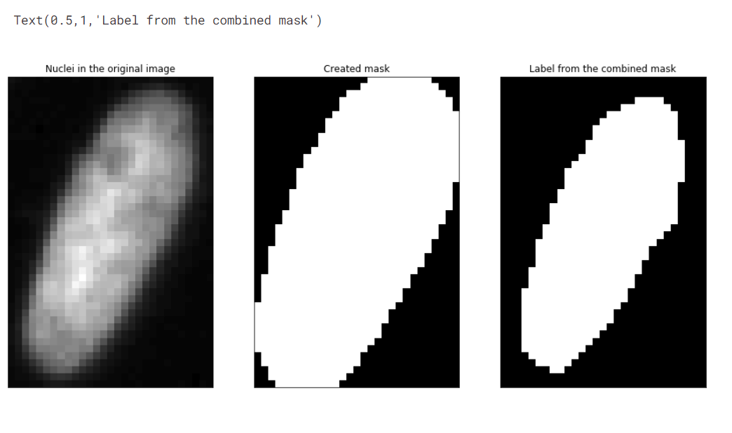bjects=ndimage.label(canny_mask)[0]
plt.figure(figsize=(16,8))
plt.subplot(1,3,1)
plt.imshow(grayimg[ndimage.find_objects(objects)[20]],cmap='gray')
plt.xticks([])
plt.yticks([])
plt.title('Nuclei in the original image')

plt.subplot(1,3,2)
plt.imshow(canny_mask[ndimage.find_objects(objects)[20]],cmap='gray')
plt.xticks([])
plt.yticks([])
plt.title('Created mask')

plt.subplot(1,3,3)
plt.imshow(combined_mask[ndimage.find_objects(objects)[20]],cmap='gray')
plt.xticks([])
plt.yticks([])
plt.title('Label from the combined mask')

Output:

#To get one dataframe for all the pixels within all the bounding boxes in an image
pixels_gs=pd.DataFrame()
columns=[]
for i in range(9):
    columns.append('pixel-'+str(i))
columns=columns+['label']
bounding=ndimage.find_objects(objects)
for bbox in bounding:
    for i in range(1,canny_mask[bbox].shape[0]-1):
        for j in range(1,canny_mask[bbox].shape[1]-1):
            pixel0=grayimg[bbox][i][j] #center pixel
            pixel1=grayimg[bbox][i-1][j-1] #top left pixel
            pixel2=grayimg[bbox][i-1][j] #pixel above the center pixel
            pixel3=grayimg[bbox][i-1][j+1] #top right pixel
            pixel4=grayimg[bbox][i][j-1] #pixel to the left of center pixel
            pixel5=grayimg[bbox][i][j+1] #pixel to the right of center pixel
            pixel6=grayimg[bbox][i+1][j-1] #bottom left pixel
            pixel7=grayimg[bbox][i+1][j] #pixel to the bottom of center pixel 
            pixel8=grayimg[bbox][i+1][j+1] #bottom right pixel
            label=combined_mask[i][j] #label of the center pixel
            neighbors = pd.Series({a:b for (a,b) in zip(columns,[pixel0,pixel1,pixel2,pixel3,pixel4,pixel5,pixel6,pixel7,pixel8,label])})
            pixels_gs = pixels_gs.append(neighbors, ignore_index=True)

#To see the head of the dataframe
pixels_gs.head()

Output: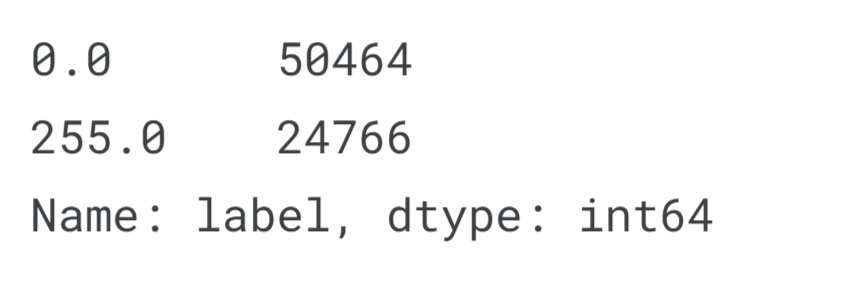

The class distribution appears to be skewed towards 0, which is unexpected when considering only pixels within the bounding boxes. This could be due to the bounding boxes encompassing larger regions than individual nuclei.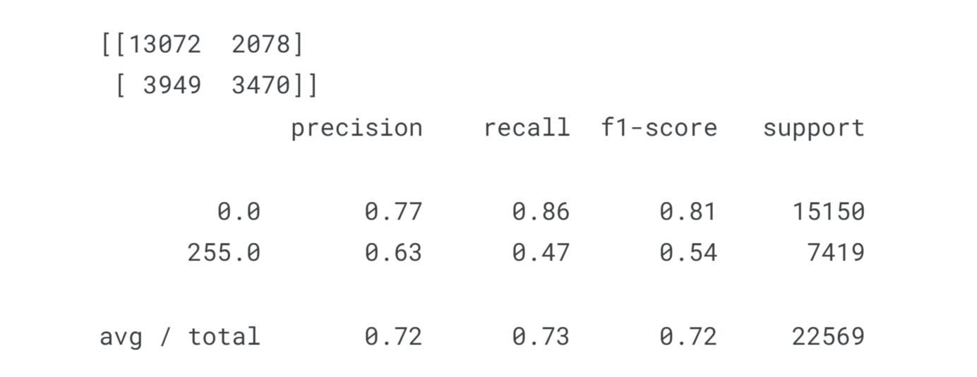

#To divide the data into training and testing sets
from sklearn.ensemble import RandomForestClassifier
from sklearn.model_selection import train_test_split

X_train,X_test,y_train,y_test=train_test_split(pixels_gs.drop('label',axis=1),pixels_gs['label'],test_size=0.3,random_state=101)
rfc=RandomForestClassifier(n_estimators=100)
rfc.fit(X_train,y_train)
rfc_pred=rfc.predict(X_test)

from sklearn.metrics import classification_report, confusion_matrix
print(confusion_matrix(y_test,rfc_pred))
print(classification_report(y_test,rfc_pred))

Output:

predicted=np.zeros((canny_mask.shape))
bbox=[]
bbox_dim_prod=[0]
rfc_pred = rfc.predict(pixels_gs.drop('label',axis=1))
for i in range(len(bounding)):
    bbox_dim=np.array(list(background[bounding[i]].shape))-2 #Since we are taking 1 to (n-1) rows and 1 to (n-1) columns
    bbox_dim_prod.append(np.product(bbox_dim)) #for indexing
    bbox_pred=rfc_pred[sum(bbox_dim_prod[0:i+1]):sum(bbox_dim_prod[0:i+1])+np.product(bbox_dim)].reshape(bbox_dim[0],bbox_dim[1]) #for reshaping the predicted labels into the reduced dimensions of the bounding box 
    bbox.append(bbox_pred)
    predicted[bounding[i]][1:predicted[bounding[i]].shape[0]-1,1:predicted[bounding[i]].shape[1]-1]=bbox[i]

plt.figure(figsize=(13,7))
plt.subplot(1,2,1)
plt.imshow(combined_mask,cmap='gray')
plt.title('Combined Mask')
plt.xticks([])
plt.yticks([])

plt.subplot(1,2,2)
plt.imshow(predicted,cmap='gray')
plt.title('Predicted Mask')
plt.xticks([])
plt.yticks([])

Output: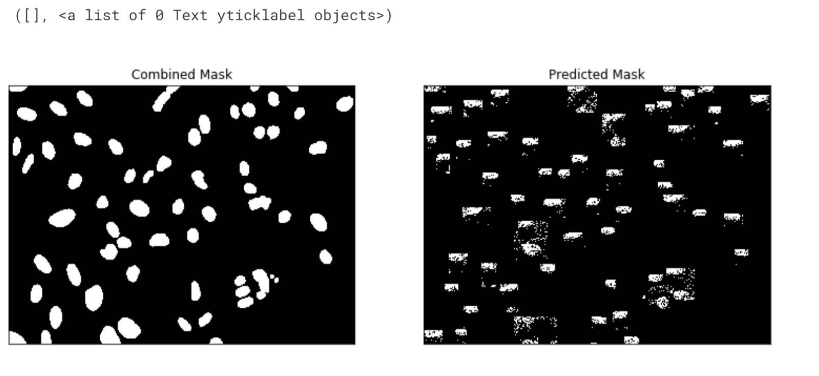

The performance of the pixel classifier depends on the defined features. It's important to note that we have trained and tested the classifier on the same image, which could lead to overfitting. To improve performance, we can consider training the classifier on pixels within bounding boxes from all training images. Additionally, using a 5x5 window and incorporating features such as the distance between the pixel and the nucleus centre or the relative density of white pixels (255 or 1s) within the defined window on the canny mask could enhance our results.

Conclusion

The combination of image processing and machine learning opens up exciting possibilities in various fields. By leveraging the power of machine learning algorithms, we can extract valuable information from visual data, automate image analysis tasks, and enhance decision-making processes. As researchers continue to innovate and refine machine learning techniques in image processing, we can expect further advancements that will transform how we interact with and derive insights from visual data.

Next TopicMachine Learning in Banking

← prev next →